Table of Contents

What is surface free energy (SFE)?
An important application of the contact angle measurement is to determine a solid-surface’s characteristic surface free energy (SFE). Picture a single molecule in a drop of liquid. The molecule is surrounded by a homogeneous environment and will experience cohesive forces from adjacent molecules, causing the molecule to tend to stay in the bulk. As we move toward the surface of the liquid where it is in contact with another phase, the molecule will experience cohesive forces toward the bulk but also some weaker adhesive forces toward the adjacent phase. The result is a net attraction into the bulk that tends to reduce the number of molecules at the surface and increase the intermolecular space between surface molecules. The increased separation requires energy, just like when stretching a spring, and this excess energy gives rise to surface tension and surface free energy (SFE).
Surface tension and SFE are mathematically equivalent but subtly different in their interpretation of the surface. Surface tension is a tension force per length acting in all directions along the surface, and its common units are mN/m or dyn/cm. SFE is interpreted as the energy required to create new surface area, and its common units are mJ/m2 (equivalent to mN/m). The SFE of a solid-vapor surface is a critical property dictating how a liquid will wet the surface. Understanding SFE is important in many applications including coatings, water repellent fabrics, enhanced oil recovery, and much more.

How is surface free energy measured with Optical Tensiometry?
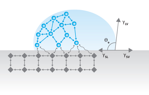
One common method for measuring SFE is by measuring the contact angles of several sessile droplets of standard liquids resting on the solid surface of interest. The static contact angle (Figure 1) is an indication of the balance of surface tensions between the liquid and solid (γSL), liquid and gas (γLV), and solid and gas (γSV), as described by the Young equation [1],
γlv cosθ = γSV – γSl
Equation 1
The visual simplicity of Equation 1 is deceptive. First, the equation assumes a smooth homogeneous surface and the entire system is in a thermodynamic equilibrium. Second, each surface tension can be considered the sum of a number of components representing different intermolecular forces:
γLV = γLVd + γLVp + γLVh + γLVi + γLVab + γo
where d, p, h, i, and ab respectively represent the dispersion, polar, hydrogen-bonding, induction, and acid-base interactions. The γo represents additional interactions. This concept was proposed by F.M. Fowkes [2].
To use Equation 1 and measured contact angles to determine SFE will require another equation. While there are a number of approaches, several of the most common ones are discussed below.
The Extended Fowkes or OWRK method (geometric mean)
As discussed above, a liquid molecule at a solid-liquid interface will experience cohesive forces from its like-molecules toward the bulk, and adhesive forces from molecules in the solid. Due to the force imbalance, there’s a difference in energy required for the molecule to reside at this surface rather than in the bulk. While Fowkes originally only considered that London dispersion forces contribute to this excess energy [2], Owens and Wendt later also considered polar interactions [3]. Using a geometric mean approach, this energy difference for the liquid molecule to reside at the surface can be expressed as:
ΔEL = γLV – √(γLVd γSVd ) – √(γLVp γSVp)
Equation 2
A similar expression for the energy difference for a solid molecule to reside at the surface can also be found. Summing these energy differences for both a liquid and solid molecule residing at the surface gives the total energy required to form a new surface,
γSL = γLV + γSV – 2√(γLVd γSVd ) – √(γLVp γSVp)
Equation 3
After combining Equation 3 with Equation 1, the OWRK equation is found:
γLV(1+cosθ) = 2(√(γLVd γSVd ) + √(γLVp γSVp ))
Equation 4
Equation 5 is used to find two unknowns, γSVd and γSVp, and thus contact angle measurements with at least two liquids with known γLVd and γLVp are needed. One liquid should be dominantly polar (e.g. water or glycerol) and one liquid should be dispersive (e.g. diiodomethane). Afterward the total surface free energy of the solid-liquid surface is γSV=γSVd + γSVp. The OWRK method is one of the more common approaches to determining the surface free energy of solids using contact angle measurements.
The Wu method (harmonic mean)
S. Wu and K.J. Brzozowski proposed a reciprocal or harmonic mean as opposed to the geometric mean, claiming the geometric mean approach is not applicable to polar-polar systems [4]. In this case, the energy to create the new surface is
γSL |
= |
γSV + γLV – 4 |
[ |
γSVd γLVd |
+ |
γSVp γLVp |
] |
|||
γSVd + γLVd |
γSVp + γLVp |
|||||||||
Equation 5
And, when combined with Equation 1, the Wu equation becomes
γLV(1+cosθ) |
= |
4 |
[ |
γSVd γLVd |
+ |
γSVp γLVp |
] |
|||
γSVd + γLVd |
γSVp + γLVp |
|||||||||
Equation 6
Like with the OWRK method, two liquids – one polar and one dispersive – are needed to measure the SFE. In practice the OWRK is generally more accurate than the Wu method.
The Van Oss-Chaudhury-Good method (acid-base)
C.J. Van Oss, M.K. Chaudhury, and R.J. Good developed a more advanced approach based on the Lifshitz theory of attraction between macroscopic bodies [5]. They proposed that the solid SFE consists of two terms: the Lifshitz-van der Waals interactions, γLW, consisting of dispersion, polar, and induction interactions; and the acid-base interactions, γa and γb, where a indicates acid and b indicates base. In this approach, the SFE is calculated using:
γLV(1+cosθ) = 2(√(γLVLW γSVLW ) + √(γLVb γSVa ) + √(γLVa γSVb ))
Since the Van Oss-Chaudhury-Good method has three unknowns, γSVLW, γSVa and γSVb, three contact angle measurements with three liquids are required: one dispersive liquid (e.g. diiodomethane), and two polar liquids (e.g. water and glycerol). While this approach has the potential to lend more in-depth insight into the surface properties, sometimes negative square roots appear, which have not received a proper explanation, leading to a number of objections to the theory [6].
How is surface free energy measured with Force Tensiometry?
Surface Free Energy can also be determined via Force Tensiometry contact angle measurements. However, these SFE values are not the same as SFE determined by optical tensiometry. Since force tensiometers cannot measure static contact angle, SFE measurements using Force Tensiometry are calculated using advancing and receding (dynamic) contact angle measurements only. Thus, the results of a force tensiometry SFE calculation cannot be directly compared with those obtained by using an optical tensiometer and several static contact angle measurements. Among other differences, SFE determined by force tensiometry can use a variety of different contact angles for the calculations, with some using only the advancing value and others relying upon both advancing and receding values.
The force tensiometry SFE technique is advantageous to use in cases where a static or sessile drop measurement is not possible. For example, it is much easier to determine the SFE of irregular samples such as individual fibers, powders, and wires using force tensiometry. Another benefit of using force tensiometry to determine SFE is that the calculated values provide an average over the entire surface area of the sample that is immersed in the probe liquid, rather than on a few specific locations on a sample that may or may not be homogeneous.
Surface Free Energy on Non-Ideal Surfaces
Each of the SFE theories discussed in this article is based on Young’s equation, hence, they must adhere to the same assumptions about the surface and its properties. However, it is well known that in practice, at least one of these assumptions is typically violated in any given experiment. Therefore, it is sometimes beneficial to use corrected-contact angle measurements to determine the SFE of a surface. Taking into account the chemical or topographical heterogeneity of a sample ensures that the calculated SFE values are not skewed by inconsistencies in the surface material. This is especially applicable when using SFE as measure of success for surface treatments or coatings. Our Contact Angle and Wettability technique page provides more detailed information about corrected contact angle and how to implement this practice in your experiments: Contact Angle Measurements and Wettability
References
[1] P.C Hiemenz, R. Rajagopalan. “Principles of Surface and Colloids Chemistry.” Taylor & Francis Group, Boca Raton, FL, 1997.
[2] F.M. Fowkes. Attractive forces at interfaces. Ind. Eng. Chem. 56 (1964) 40–52.
[3] D.K. Owens, R.C. Wendt. Estimation of the surface free energy of polymers. J. Appl. Polym. Sci. 13 (1969) 1741-1747.
[4] S. Wu, K.J. Brzozowski. Surface free energy and polarity of organic pigments. J. Colloid. Interface Sci. 37 (1971) 686-690.
[5] C.J. van Oss, M.K. Chaudhury, R.J. Good. Interfacial Lifshiz-van der Waals and polar interactions in macroscopic systems. Chem. Rev. 88 (1988) 927-941.
[6] H.Y. Erbil. The debate on the dependence of apparent contact angles on drop contact area or three-phase contact line: A review. Surf. Sci. Rep. 69 (2014) 325-365.
Lorem ipsum dolor sit amet, consectetur adipiscing elit. Ut elit tellus, luctus nec ullamcorper mattis, pulvinar dapibus leo.