Introduction
Plastics made from polymeric materials are an integral part of many consumer goods and products. Whether it is the packaging or the product itself, different polymers can provide material and mechanical properties to suit the product’s functional needs. With the increased integration of environmentally sustainable polymers along with concerns over the recyclability of conventional plastics, polymer blends may be sought after to achieve ideal performance properties while wholly unavoidable when recycling products that contain multiple polymers. The challenge with polymer blends is that many polymers form an incompatible final structure. In fact, two of the most common consumer-based polymers polypropylene and polyethylene, when mixed, can have poor impact resistance and interfacial adhesion [1,2]. To avoid this, additional polymeric ‘compatibilizers’ may be added to improve the miscibility. Therefore, methods are needed to quickly and easily determine if polymers can form compatible mixtures or which compatibilizers will most improve the final blend.
Characterizing the Surface with Contact Angle Measurements
A simple and effective way to characterize and predict the compatibility of two or more polymers is through contact angle measurements with an optical tensiometer coupled with surface free energy modeling. An optical tensiometer operates by placing liquid drops (usually water and diiodomethane) onto a solid sample surface (our polymers of interest), recording images of the droplet structure on the surface, and analyzing the angle of liquid contact from the droplet’s edges. From the contact angle values and the known surface tensions of the probe liquids, we can determine the surface free energy (SFE) of the sample. SFE is analogous to the surface tension of the solid sample surface and is a powerful descriptor of the types solid and liquid interactions, like adhesion and mixing, that a material is capable of. The most widely used and recommended SFE model is the OWRK-Fowkes method, which gives us the overall SFE value (γtotal) and the contributions from the individual polar (γsvp) and dispersive (γsvd) surface tension components [3,4].
SFE and Beyond: Interfacial Tension and Spreading Coefficients
After contact angle measurements are taken on the sample surface, the liquid’s polar (γlvp) and dispersive components (γlvd) are used to calculate the corresponding SFE components of the surface (Equation 1).
√γsvp γlvp + √γsvd γlvd = 0.5γlv(1 + cosθ)
Equation 1
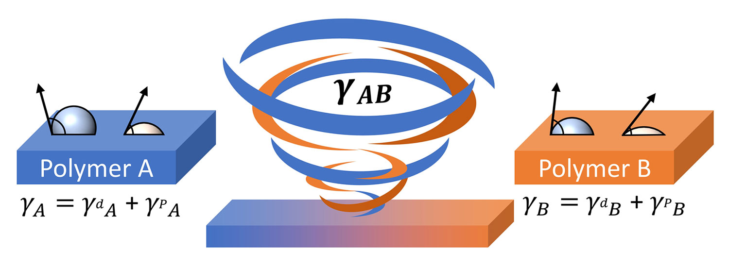
While these values alone reveal information about a surface’s properties, they can be further utilized to quantify the compatibility of two different polymers. This is accomplished by finding the geometric (or sometimes harmonic) mean between two sets of SFE values, giving us the interfacial tension, γAB, for a polymer A and polymer B (Equation 2) [4,5].
γAB = γA + γB– 2(γAp γBp )0.5 – 2(γAd γBd)0.5
Equation 2
In general, it is found that the lower the measured interfacial tension between two polymers, the higher the miscibility and the better the blending. If the interfacial tension of two polymers is high, then a third polymer can be added as a “compatibilizer” to increase the miscibility of the original two polymers. The same SFE measurements can be used with the compatibilizer material (polymer C) to then calculate the interfacial tension between the polymers and the compatibilizer. For an effective compatibilizer, the interfacial tension should have values lower with the compatibilizer than with the original two polymers (γAC<γAB & γBC<γAB) [6].
These measured interfacial tension values can also be used to predict the final morphology of polymer blends, even when it is a ternary mixture like with a two-component polymer plus a third polymer component compatibilizer. Using the surface free energy and interfacial tension values, the spreading coefficient can be calculated to determine how the polymers will interact in the final matrix [7]. The spreading coefficient (spreading coefficient=λ where λAB represents the spreading of substance A over B) is traditionally a quantity associated with how well a liquid spreads across a solid surface. This coefficient is calculated by determining the difference between the interfacial tension of the liquid-solid interface and the individual surface tension of the liquid and the surface free energy of the solid (Equation 3).
λAB = γB – γA – γAB
Equation 3
If the coefficient is positive, then the tendency of the liquid is to spread and form a film on the surface, while a negative value indicates that the liquid will form a finite droplet. With a spreading coefficient of zero, the liquid is not considered wetting nor nonwetting. The physical basis of Equation 3 can be described with the following: spreading of A over B is favored when the adhesive force (high adhesion occurs when the γAB is small) between the two phases is greater than the cohesive force (low cohesion occurs when γA is small) of the spreading liquid.
With polymer melt blends, Hobbes spreading theory can be employed, using the interfacial tension between the components of a ternary polymer mixture to calculate each spreading coefficient (Figure 1, top half) and then predict which polymer interactions are favored in the resulting final polymer structure. Depending on the sign and magnitude of each spreading coefficient, the polymer blend can have the morphologies observed in the bottom half of Figure 1: full phase separation, different core-shell encapsulations, or a partial encapsulation. To observe full phase separation based on polymer matrix A/B/C in Figure 1, the spreading of A over B and/or C (λAB>0 or λAC>0) needs to be favored over the spreading of B over C and C over B (λBC<0 and λCB<0). For core-shell phases to occur, the spreading of polymer A over B or C should be unfavored (λAB<0 or λAC<0) with favored spreading of B over C or C over B (λBC>0 and λCB>0). Partial encapsulation can occur when the spreading coefficient for all scenarios is positive ((λAB>0 or λAC>0; λBC>0 and λCB>0), as all phases will have some favorable interaction.
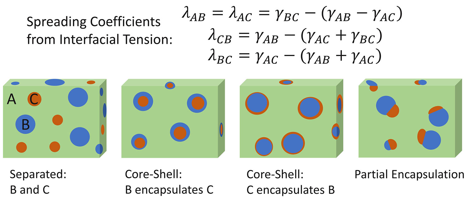
From the spreading coefficient, the morphology of something like a recycled plastic container with multiple polymers can be predicted. Both the interfacial tension measurements and spreading coefficient values taken from contact angle measurements have been used in recent publications to improve polymer mixtures. This treatment has been done to find effective compatibilizers for common plastics like polyethylene and polypropylene, as well as create effective blends of fully biodegradable polymers [6,8].
Wetting and Adhesion Analysis with OneAttension Software for IFT/Spreading Coefficient
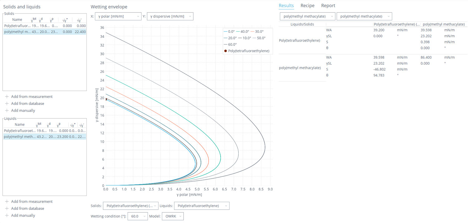
While some calculations are involved in going from liquid-based contact angle measurements to spreading coefficients, this does not have to be difficult. With the OneAttension software with the Theta optical tensiometers, after the software fits and measures the contact angle images of the probe liquids, this information is automatically fed into multiple SFE models, including the OWRK-Fowkes model, giving us the surface’s total SFE and individual polar and dispersive components. These can then be opened with the Wetting and Adhesion Analysis (WAA) module, included with the OneAttension software, and used to analyze our different surface properties (screenshot shown in Figure 2). The SFE values from the contact angle measurements, or values manually entered in or from the solid/liquid databases, can then be converted to an arsenal of wetting and adhesion-based tools. For more traditional liquid/solid analysis, wetting envelope graphs are created, which depict contact angles of the liquid as a function of the relative polarity/dispersiveness of the liquid and solid. This can be useful in formulating liquid coatings and managing surface treatments to dial in effective adhesion.
Beyond the wetting envelope, the WAA package allows us to access key properties to understand polymer blend propensities using contact angle measurements quickly and easily. From contact angles on the different polymer surfaces, the calculated SFE values can be selected to automatically provide the interfacial tensions, spreading coefficients, and work of adhesion between the different polymers. Like with the treatment of the ternary polymer mixture in Figure 1, these values can then be used to compare and predict the mixing, morphologies, and necessity of additional compatibilizers for the polymer blends.
References
[1] J. Polym. Sci. Part B Polym. Phys. 2000, 38, 108–121
[2] Polymer 2004, 45, 893–903
[3] Fowkes, F.M.; Industrial and Engineering Chemistry, 56, 12, 1964.
[4] Owens, D.K.; Wendt, R.C.; Jour. Of Applied Polymer Science, 13, 1741, 1969.
[5] Wu, S. J. Polym. Sci. Part C Polym. Symp. 1971, 34, 19–30
[6] Polymers 2021, 13, 3567
[7] POLYMER, 1988, Vol 29, September
[8] Materials Today Sustainability 21 (2023) 100314