Surface Tension, Surface Free Energy, and Wettability

What Does Surface Free Energy Tell Us?

The surface free energy (SFE) of a solid surface can tell you a lot about how different liquids will interact with said surface. In our surface free energy technique page, we discussed how the SFE of a solid can be calculated from contact angle measurements using several models including the commonly used Owens-Wendt-Rabel-Kaelble (OWRK) model. But once you measure the SFE, the next logical question is “what can I do with this information?” In fact, the OWRK model can be a powerful tool to predict wettability and adhesion based on the SFE and liquid surface tension, and it can help guide your research and development. In this page we will introduce wetting envelopes as a convenient visualization tool, and explain the relationships between SFE, surface tension, and contact angles.

The Owens-Wendt-Rabel-Kaelble (OWRK) Model

In these analyses it is common to use the OWRK model, where the liquid surface tension, γ_LV, is a sum of a dispersive component (γ^D_LV e.g. London dispersion forces) and polar component (γ^P_LV, e.g. hydrogen bonding) such that γ_LV = γ^D_LV + γ^P_LV. Likewise, the solid SFE, γ_SV, is a sum of dispersive and polar components such that γ_SV = γ^D_SV + γ^P_SV. Then the relationship between liquid surface tension, solid SFE, and the contact angle between the liquid and the solid is described by the OWRK equation:

(1)

where θ is the contact angle between the liquid and the solid. Some important assumptions are made in the OWRK model: the liquid is pure, the solid is smooth and chemically homogenous, and there are no chemical reactions between the liquid and the solid. No real system will completely satisfy all of these assumptions, but nontheless the OWRK model is a powerful model that is widely used in industry and academia to guide material selection.

What is a Wetting Envelope?

Liquid surface tension, solid SFE, and the contact angle a liquid droplet makes on the surface are all related. The wetting envelope helps us visualize these relationships and can help us better understand our system and choose materials.

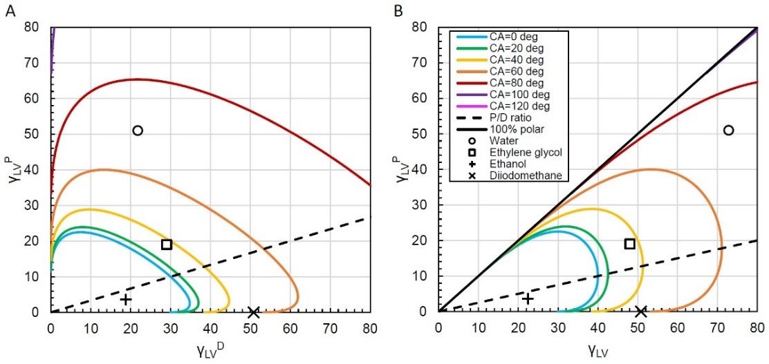
Figure 1 shows wetting envelope contour plots for a theoretical solid with γ^D_SV = 30 mN/m and γ^P_SV=10 mN/m. This means the polar ratio is γ^P_LV / γ_LV = 0.25 and the dispersive ratio is γ^D_LV ⁄ γ_LV = 0.75. In both plots, the solid colored lines are isolines with a fixed angle θ, meaning if you travel along any line then θ will stay the same. In Fig. 1A, the vertical axis represents changing with γ^P_LV, while the horizontal axis represents changing with γ^D_LV. In figure 1B, the horizontal axis represents changing the total surface tension with γ_LV instead. Both plots represent the same system with the same isolines. The style of figure 1A tends to be more common in the literature, but figure 1B may be more convenient if you prefer to visualize wettability in terms of with γ_LV and with γ^P_LV.

These plots are particularly useful when interpreting how changing polar and dispersive components of liquid surface tension will affect θ. For example, in figure 1B, consider a liquid with total surface tension γ_LV = 40 mN/m and γ^P_LV = 0 mN/m (meaning γ^D_LV = 40 mN/m). The contact angle begins close to 40° as indicated by the yellow isoline. Now increase γ^P_LV by moving vertically in the plot, and you will notice that θ starts decreasing. At γ^P_LV=10 mN/m, we reach a point where the polar and dispersive ratio of the liquid surface tension matches the polar and dispersive ratio of the solid, represented by the dashed black line. At this point, θ is minimized for a given γ_LV, and if we continue to increase γ^P_LV past 10 mN/m you will see θ start to increase again.

Using these wetting envelopes, two key concepts related to how surface tension affects contact angles are visualized. First, for a given γ_LV, the contact angle will be minimized if the polar and dispersive ratios of the liquid surface tension match those of the solid SFE. We can see this by looking at the coordinates in figure 1 representing ethylene glycol (γ_LV = 48 mN/m) and diiodomethane (γ_LV = 50.8 mN/m). Both liquids have similar total surface tensions, but the plots indicate diiodomethane will have a contact angle around 60° whereas ethylene glycol will be just below 40°. This is because the polar and dispersive ratio of ethylene glycol is a better match to the solid SFE polar and dispersive ratios.

The second concept is that if γ_LV is low enough, the polar and dispersive ratios might not make much difference. Take the point in figure 1 representing ethanol with γ_LV = 22.4 mN/m. The wetting envelope indicates that θ = 0° or there is perfect wetting, and if we change the polar and dispersive ratio we would still have perfect wetting simply because γ_LV is so low.

Figure 1 – Wetting envelope plots for a solid with γ^D_SV=30 mN/m and γ^P_SV=10 mN/m. In (A) the horizontal axis is the dispersive surface tension component γ^D_LV, and in (B) the horizontal axis is the total surface tension γ_LV. Points representing water, ethylene glycol, ethanol, and diiodomethane are plotted.

How Can We Use Surface Free Energy and Wetting Envelopes to Understand Wettability?

Using our knowledge of wetting envelopes and the relationships between surface tension, surface free energy, and contact angles, we can intelligently approach various research and development problems. Whether your goal is to increase wettability (decrease θ) or decrease wettability (increase θ), our options are to modify the solid or modify the liquid.

If our plan is to modify the liquid to increase wettability, or goals should include one or both of (a) get the polar ratio γ^P_LV ⁄ γ_LV and dispersive ratio γ^D_LV ⁄ γ_LV closer to that of the solid, and/or (b) reduce the total surface tension. In the previous section we looked at how changing the liquid properties influenced the contact angle on a specific solid substrate.

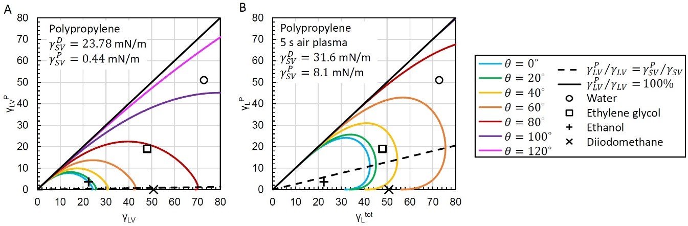
In many cases, the liquid may be fixed or difficult to sufficiently modify, and it is easier to manipulate the solid’s properties. A good example of this are applications involving the coating of polymers like polypropylene. Polypropylene is a widely used polymer due to its good chemical resistance, machinability, and relatively low cost, but it is naturally hydrophobic and is difficult to wet with many liquids. A wetting envelope of untreated polypropylene is shown in figure 2A, and due to its low SFE and being primarily dispersive, it is clear from this visualization that few liquids will wet the material well. Even ethanol with its low surface tension will have a nonzero contact angle on polypropylene.

However, the SFE of polypropylene is easily manipulated by plasma treatment, and in the application note “Enhanced Wettability Plasma Treated Polypropylene we demonstrated that there is an optimal treatment time to get the best SFE properties for wetting. By plotting the wetting envelope of polypropylene after a 5 s air plasma treatment in figure 2 B, you can see that the total SFE was increased, but the polar component was also significantly increased, providing better wettability for liquids with significant polar fractions like water and ethylene glycol. This allows a liquid like ethylene glycol to decrease its contact angle from just under 80° on untreated polypropylene (figure 2 B) to <40° on plasma treated polypropylene (figure 2 A and B respectively).

Figure 2 – Wetting envelopes for (A) untreated polypropylene and (B) polypropylene after a 5 s air plasma treatment. All SFE measurements were made at Nanoscience Analytical using an Attension Theta Flex optical tensiometer.

How Can You Make a Wetting Envelope Plot?

Wetting envelope plots are very useful tools, and they do not require anything more complicated than Microsoft Excel to create. We begin with the OWRK equation but rewrite it using polar coordinates.

Figure 3 – Polar coordinate system used for making a wetting envelope plot.

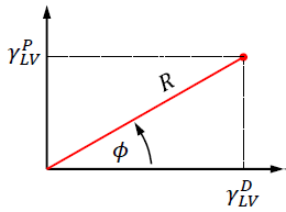
In the polar coordinate system in Fig. 3, the γ^D_LV and γ^P_LV coordinates used in figure 1A are described by the angle Φ and the radius R, where:

(2) γ^D = R cosΦ,

(3) γ^P = R sinΦ

In the OWRK model, this means that the total surface tension in this polar coordinate system is γ_LV=R cos⁡ϕ+R sin⁡ϕ. Using these relationships, it is a simple matter of inserting them into the OWRK equation,

(4)

and then solving for the radius R,

(5)

For a given θ, γ^D_SV and γ^P_SV, it is straightforward to calculate R(ϕ) over the range 0^∘ ≤ ϕ ≤ 90^∘, and then it is a simple matter of using equation (2) and (3) to determine γ^D_LV and γ^P_LV. This produces one isoline at the level θ. Then, by repeating the process for multiple θ, you can construct a wetting envelope contour plot to visualize your system and play with different liquid or solid properties.

List of Symbols and Their Definitions

• γ_LV : Total liquid-vapor tension, where γ_LV = γ^P_LV + γ^D_LV
• γ^P_LV : Polar component of the liquid-vapor surface tension
• γ^D_LV : Dispersive component of the liquid-vapor surface tension
• γ_SV : Total solid-vapor surface free energy, where γ_SV = γ^P_SV + γ^D_SV
• γ^P_SV : Polar component of the solid-vapor surface free energy
• γ^D_SV : Dispersive component of the solid-vapor surface free energy
• ϕ : Contact agnel of a liquid drop on a solid surface
• Φ : Angular coordinate in the polar coordinate system used to make a wetting envelope plot
• R : Radial coordinate in the polor coordiante system used to make a wetting envelope plot