How to Prepare & Characterize Solutions for Electrospinning

Reproducibility and batch-to-batch consistency

For infrequent users or researchers working with home-built units, electrospinning and electrospraying can appear to have difficulties with reproducibility. When processing parameters are all globally controlled, but batch-to-batch inconsistencies are still present, sample development can become a frustrating experience. However, electrospinning and electrospraying depend on both the processing parameters and the solution being processed. A fully characterized solution that is easily reproducible is crucial for preventing process instability and minimizing sample variability.

Full solution characterization requires analyzing properties such as solid content, viscosity, surface tension, and conductivity. While not often considered, monitoring the time elapsed after mixing and homogenizing the solution also is fundamental for preventing solution variability, since solution properties can shift over time. For needle-based processes, maintaining a stable Taylor cone is essential to prevent needle clogging and improve batch-to-batch consistency.

Solution Preparation

Polymer solutions, including emulsions and suspensions, are a key component for reproducible and successful commercial products. Solutions must be properly prepared to minimize wasted material and production costs. Key steps to consider when preparing a solution for electrospinning or electrospraying include:

Standardize the Preparation Procedure

A standard operating procedure (SOP) should be established defining how to prepare the solution as well as what needs to be monitored and characterized. If possible, the SOP should follow ASTM standards for solution preparation, including ASTM D5226 (Standard Practice for Polymer Materials). Parameters that should be monitored according to this standard include polymer and solvent selection, solution concentration, temperature, time, container, heating mode and agitation speed.¹

It is imperative to keep track of details related to the polymers, solvents and additives used, including the batch number, expiration date, certificate of analysis, and any technical sheets available. This helps identify any variability between batches that will ultimately affect the solution properties. Key batch parameters to monitor include number-average molar mass (M_n), weight-average molar mass (M_w), viscosity-average molar mass (M_v) and intrinsic viscosity (IV). Also, noting the purity of a solvent and any additives (typically used as stabilizers) is crucial for process validation, as these factors could affect the solution.

Ensure the polymer is fully dissolved, well mixed, and homogeneous

Electrospinning and electrospraying solutions typically consist of a polymer and a solvent. For proper sample development, the polymer should be fully dissolved and well mixed into the solvent. If the polymer is fully dissolved but partially mixed, there will be a concentration gradient across the sample, preventing consistent fiber or particle formation. This is a common issue faced by electrospinning and electrospraying groups. To improve solution stability over time, polymers and solvents should be carefully selected to avoid chemical reactions or decomposition of either component.

To see the preparation of a fully dissolved, well mixed, and homogenous solution, consider Figure 1, which shows 10 wt% polycaprolactone (PCL; M_n ~ 80 kDa) dissolved in 1,1,1,3,3,3 hexafluoroisopropanol (HFIP) at different stages. Figure 1a shows PCL starting to dissolve in a couple minutes after the addition of HFIP. Over time, the PCL will fully dissolve as shown in Figure 1b, with a stripe-like pattern inside the vial. Those stripes are an indication that the polymer is still not fully mixed and the solution is not homogeneous. Constant stirring for 4+ hours leads to a clear, well-mixed and homogeneous solution, seen in Figure 1c. At that stage, the solution is ready to be used for sample development.

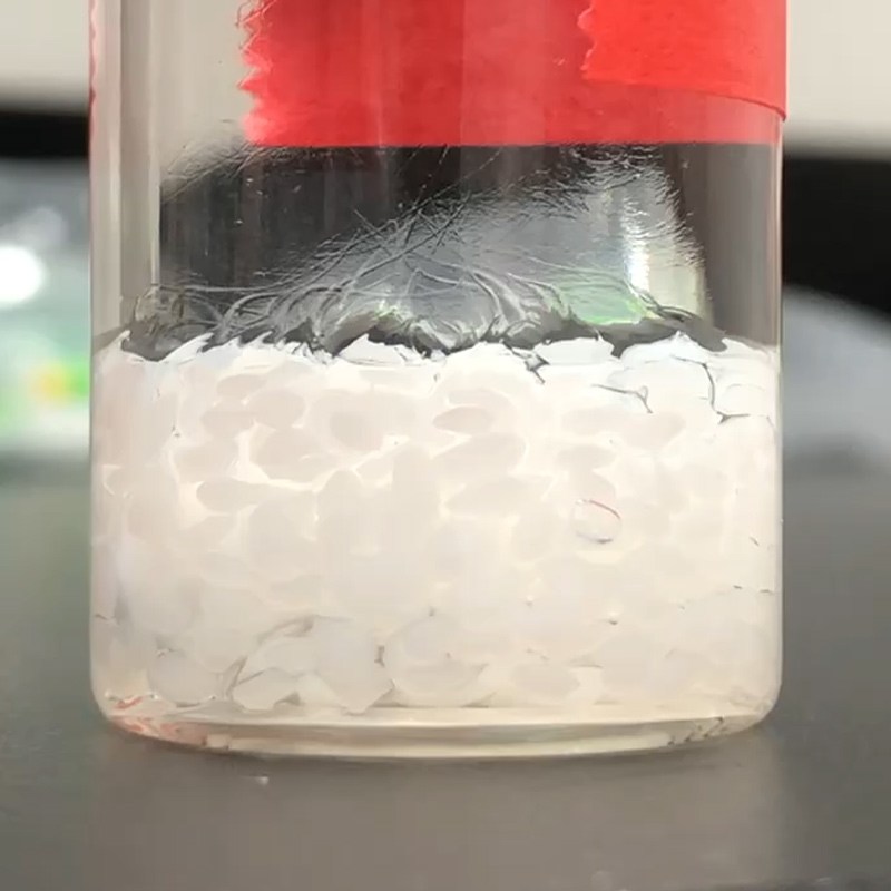
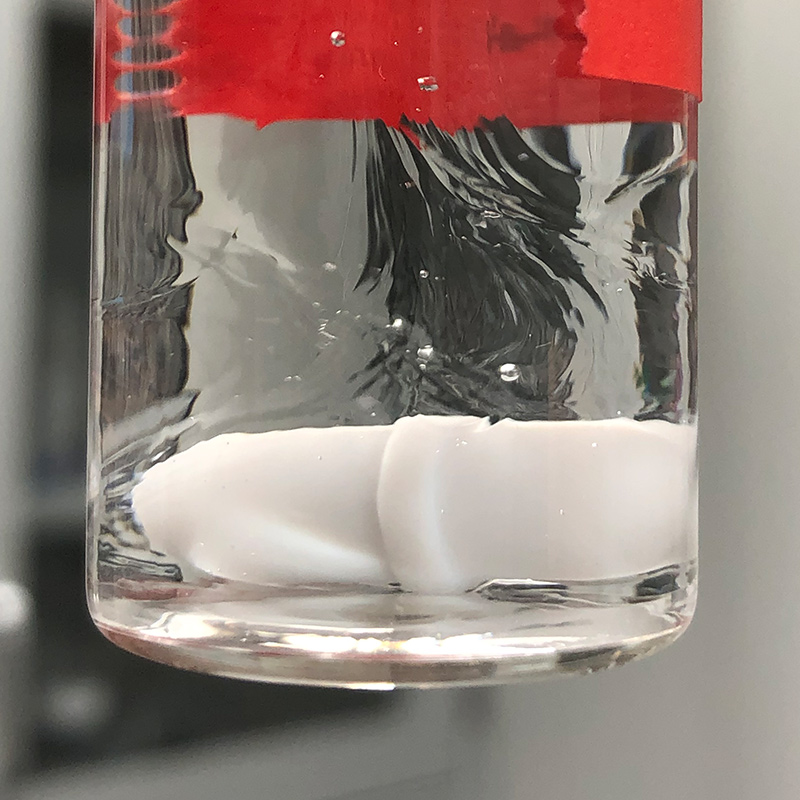
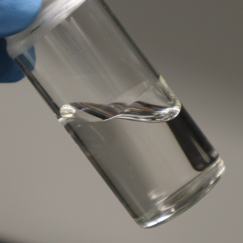
Figure 1. PCL in HFIP at a concentration of 10 wt% and at different stages during solution preparation: A) PCL starting to be solubilized by HFIP, B) PCL is fully dissolved but not well mixed and homogeneous, and C) PCL solution fully dissolved, well mixed and homogeneous.

Sometimes the use of a co-solvent is necessary to improve material solubility. Co-solvents must be miscible and unreactive with other components of the solution. Table 1 shows the most typical solvents for electrospinning and electrospraying, along with key properties used for solvent selection. The use of ionic liquids and deep eutectic solvents is becoming popular as greener alternatives to typical organic solvents. Some solutions also involve the use of a co-polymer to make the main polymer easier to spin.

Solvent name	Solvent abbreviation	Boiling point (°C)	Vapor pressure at 20°C (mmHg)	Dielectric constant	Surface tension at 20°C (mN/m)	Density at 20°C (g/mL)
Acetic acid	AA	118	11.4	6.2	27	1.049
Acetone	Ace	56	185.5	21.5	25.2	0.788
Chloroform	CHF	61	160	4.8	27.5	1.489
Cyclohexane	Cy	81	78	2.02	24.95	0.7781
N,N-Dimethylacetamide	DMAc	166	2.25	37.8	36.6	0.937
Dichloromethane	DCM	40	353	8.93	26.5	1.326
N,N-Dimethylacetamide	DMAc	166	2.25	37.8	36.6	0.937
N,N-Dimethylformamide	DMF	152	2.3	36.7	37.1	0.945
Dimethyl sulfoxide	DMSO	189	0.42	46.7	43.54	1.096
Ethanol	EtOH	78	44.63	24.5	22.1	0.789
Ethyl acetate	EA	77	73	6.0	23.9	0.901
Formic acid	FA	101	42.97	57.9	37.67	1.221
Glycerol	Gly	290	0.0002	13.2	63.4	1.261
Hexane	HX	69	124	1.9	18.43	0.659
1,1,1,3,3,3-Hexafluoro-2-propanol	HFP	58	120.01	15.7	14.7	1.596
Isopropyl alcohol	IPA	82	33	17.9	23	0.786
Methanol	MeOH	65	126.76	32.7	22.7	0.791
Methyl acetate	MA	57	216.02	8.0	24.8	0.932
N-Methyl-2-pyrrolidone	nMP	202	0.29	33.0	40.79	1.026
Tetrahydrofuran	THF	66	127	7.6	26.4	0.888
Water	W	100	18	80.3	72.8	0.998

Table 1. Common solvents used for electrospinning and electrospraying processes and their properties.²

Ensure that additives are properly suspended or dispersed

Additives can also be used in solution, emulsions, or suspensions for electrospinning and electrospraying. These additives should be fully dissolved, well mixed, and homogeneous to maintain consistent product development. If the desired additive is not soluble, additional additives like surfactants, salts, or emulsifiers can be used to prepare a well-mixed solution. Continuous mixing of the solution while processing fibers or particles is an alternative option for more stubborn solutions.

Monitor solution age

Solution stability is often overlooked by users of electrospinning and electrospraying. Depending on the vessel used to hold the solution, how the vessel is sealed, the volatility of the solvents, the stability of the polymer, and any polymer-solvent interactions, the solution will experience a change in properties over time. By standardizing the solution preparation and characterization process, any negative effects of solution aging can be minimized.

Solution Characterization

Characterizing solution properties is critical to understand how key parameters for electrospinning and electrospraying affect the final microstructure and performance of the sample, and for ensuring consistency between batches. Critical parameters to consider when characterizing solutions include solid content, viscosity, conductivity, and surface tension.

Solid content

Solution concentration can be measured in units of weight (wt%), weight by volume (w/v%), or volume by volume (v/v%). The ratio of polymers, solvents, and additives needed for a solution can be determined from the desired concentration of the final product. To minimize waste, users should calculate the quantity of solution they need to produce based on the flow rate, processing time, and system configuration (quantity of needles, tubing diameter and tubing length), with extra solution set aside for characterization purposes.

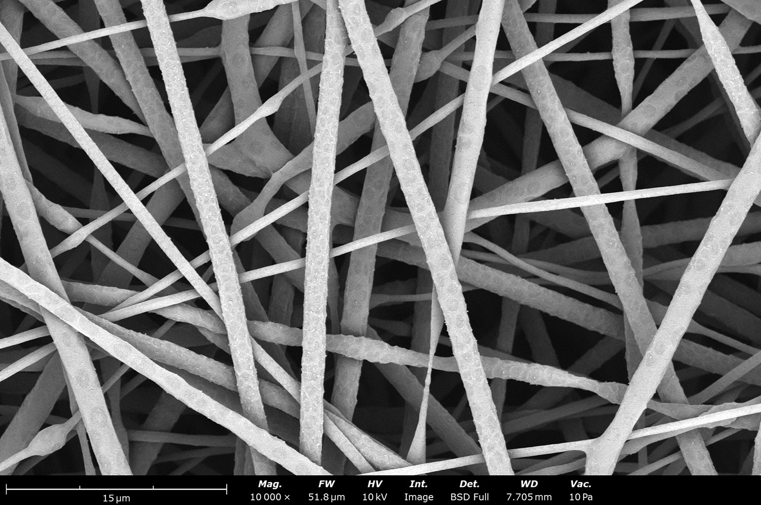
Polymer concentration is one of the primary factors affecting fiber and particle diameter. Even small changes in polymer concentration can lead to significant variations in fiber or particle morphology. An example of the microstructure of electrospun fibers at different concentrations can be seen in Figure 2, where the fibers were made with PCL in HFIP solutions. In this study, all solutions were prepared by dissolving PCL in HFIP for 18 hours at 23 °C inside a 30 mL glass vial while magnetically stirring with a 1 cm stir bar at 100 rpm angular speed. All solutions were processed with a Fluidnatek LE-50. The following parameters were kept constant between solutions: flow rate (2 mL/h), PTFE tubing (3.18 mm OD, 1.59 mm ID and 60 cm long), needle-to-collector distance (18 cm), temperature (25 ± 1°C), relative humidity (30 ± 3%), rotational speed (200 rpm on a 10 cm OD drum), substrate (polyethylene with carbon black), needle-gauge (20 Ga x 0.5 inch long), and no needle translation. Voltages were slightly optimized between solutions to maintain a stable Taylor cone during sample formation (9.0 ± 1.0 kV).

As seen in Figure 2, PCL in HFIP solutions can result in beaded fibers at low concentrations (1 and 3 wt%, Figure 2a and 2b, respectively), bimodal fiber morphology (5 and 7 wt%, Figure 2c and 2d) and uniform fiber distribution (10 wt%, Figure 2e) in the processing conditions mentioned above. Generally, higher solution concentrations (or high polymer content) lead to larger fiber diameters and a more uniform morphology, as shown in the 10 wt% PCL in HFIP sample. Figure 2f is a summary of average fiber diameter as it relates to solution concentration. The observed trend in fiber diameter is associated with an increase in polymer entanglement caused by higher viscosities when increasing polymer concentration. Similar results have been observed with PCL in chloroform (CHF),³ polyvinylidene fluoride (PVDF) in N,N-dimethylformamide (DMF),⁴ and hydroxypropyl methylcellulose (HPMC) in ethanol:water (EtOH:W).⁵

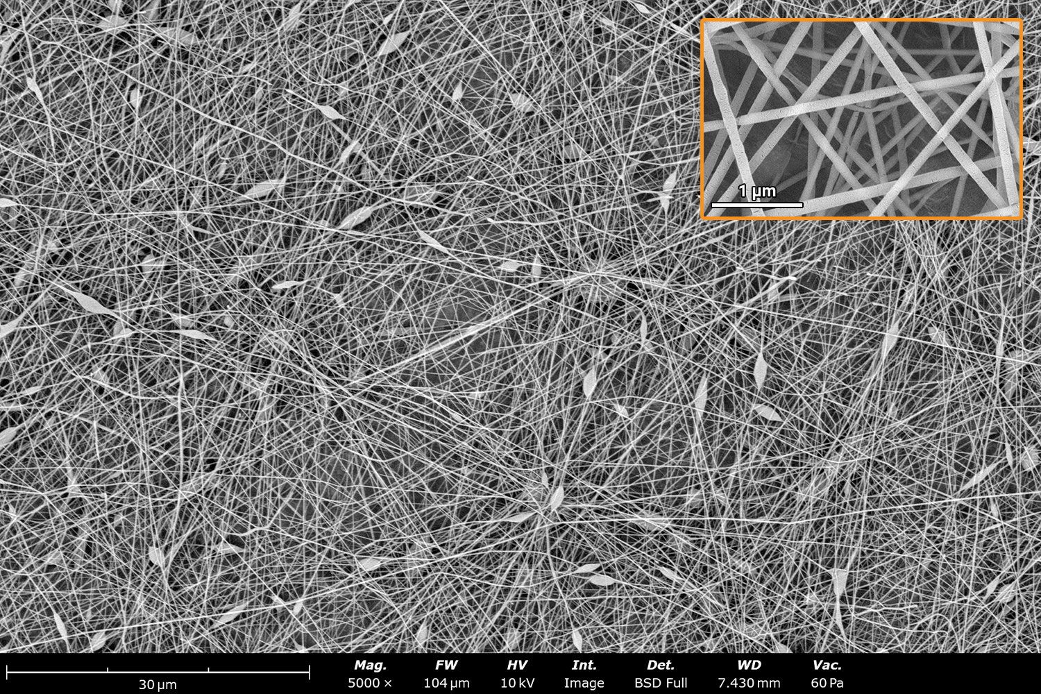
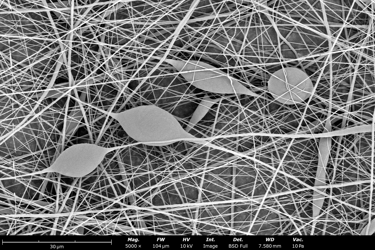
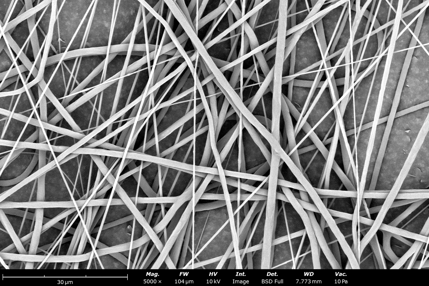
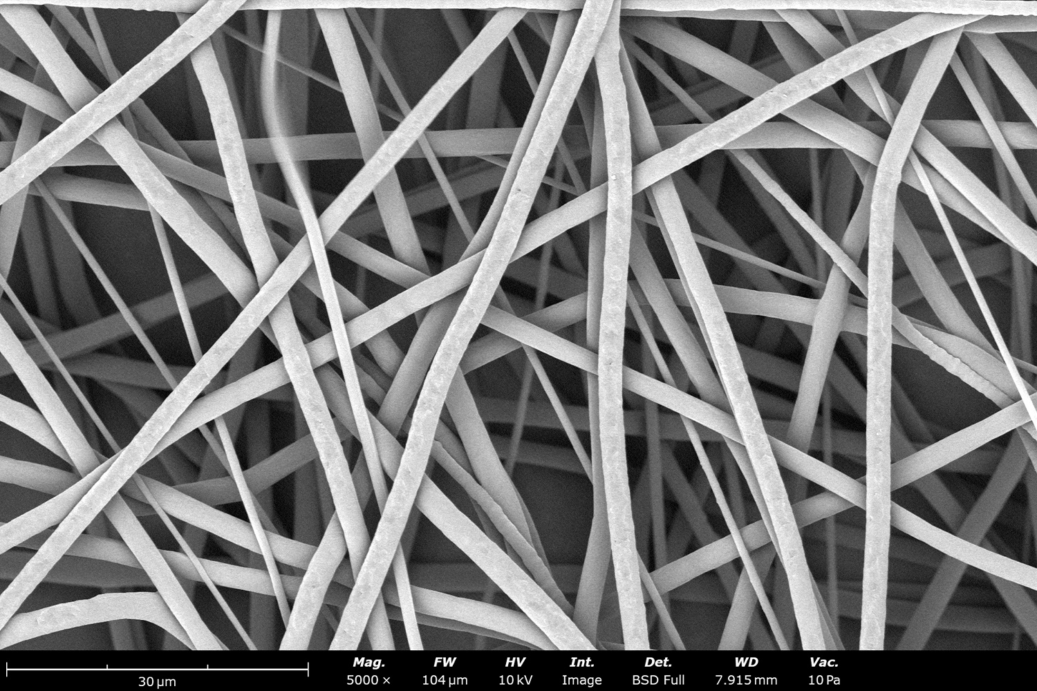
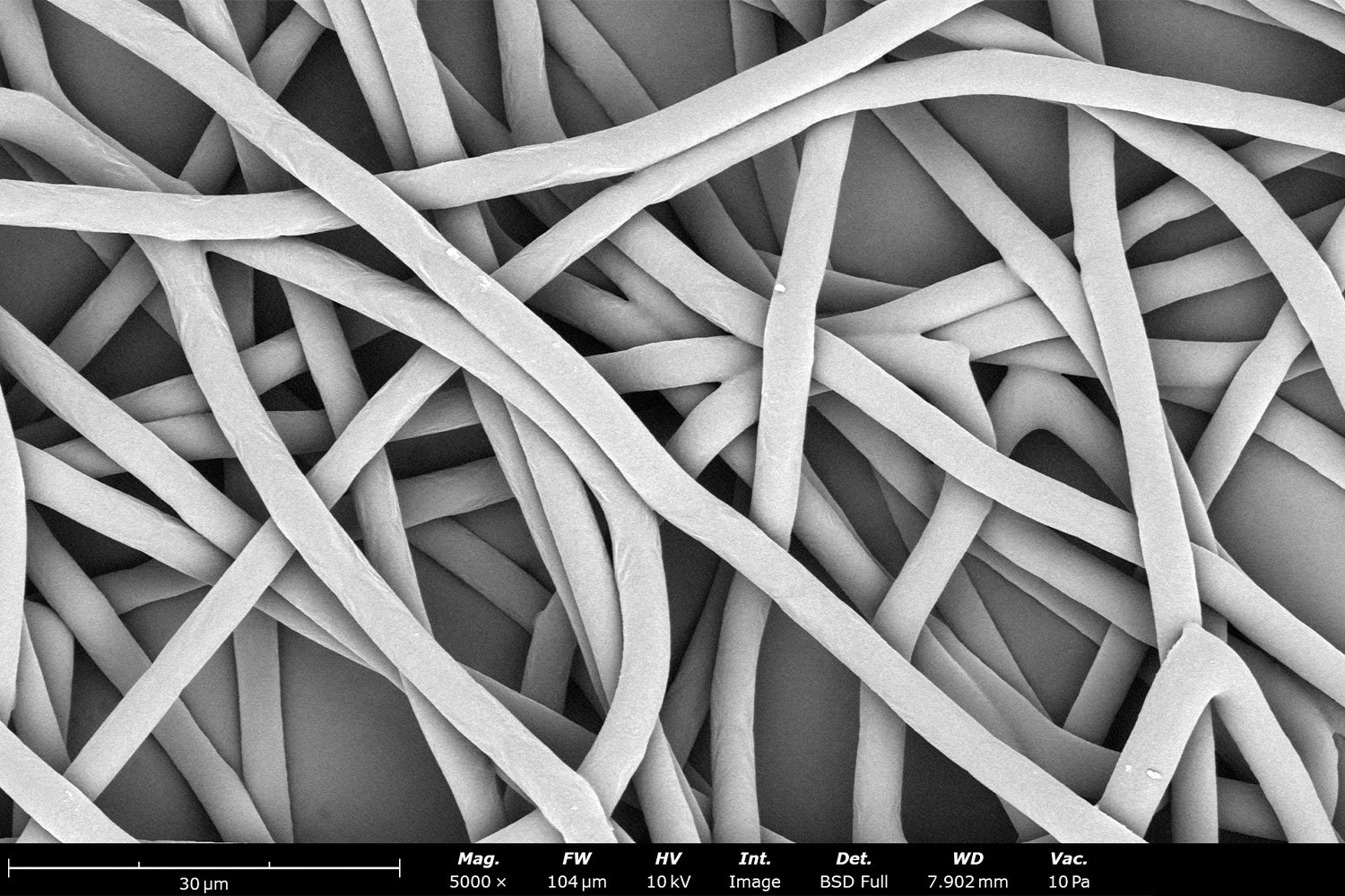
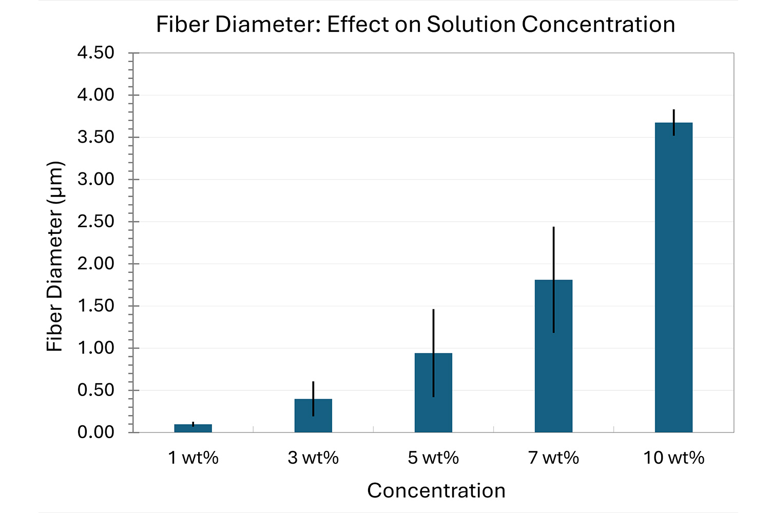
Figure 2. Effect of solution concentration on fiber diameter using PCL (Mn ~ 80 kDa) in HFIP solutions: a) 1 wt%, b) 3 wt%, c) 5 wt%, d) 7 wt%, e) 10 wt%, all at a magnification of 5,000 X; scale bar of inset image is 1 µm, and f) average fiber diameter analysis [beads not included for 1 wt% and 3 wt% analysis].

Fiber diameter is also affected by the molecular weight of the polymer, with higher molecular weights resulting in larger fiber diameters if all other parameters are kept constant. Choosing a solvent that is highly volatile is another way to achieve larger fibers or particles. With multiple factors affecting the fiber size, characterizing the solution is crucial to confirm that the concentration is within a preset average and standard deviation. This will minimize variability between users. One method of measuring concentration is using a moisture analyzer, which quantifies solid content in a solution; once the solution is fully dissolved, well mixed, and homogenous, a specific volume of it is heated to evaporate all solvents and isolate the solids.

Viscosity

Viscosity is a property of fluids that defines their resistance to flow, or in simple terms, how ‘thick’ the fluid is. Fluids with higher viscosities experience more resistance to flow. This is due to the packing density of molecules in the fluid, which makes it difficult to move past each other. Most common polymer solutions are considered non-Newtonian, meaning their shear viscosity can change as a function of the shear rate applied (the rate on how quickly a polymer solution is deformed). Conversely, a Newtonian liquid has a constant shear viscosity independently of the shear rate used, such as water or mineral oil.^6,7

Viscosity is a rheological property that is key for any polymer solution and understanding it properly is crucial for electrospinning and electrospraying processes. Properties that affect viscosity include the molar mass of the polymer, the polymer’s functional groups, solution concentration, solvent selection, processing temperature, additives in the solution, and solution age.^6,7,8,9Consider the example shown in Figure 3, which shows changes in viscosities based on the concentration of PCL in HFIP solutions. Here we see the time required for each solution to flow and relax once tilted to a 60-degree angle. As expected, viscosity and concentration are proportionally related; increasing solution concentration results in increased viscosity due to enhanced polymer chain entanglement.

Figure 3. Viscosity of PCL (M_n ~ 80 kDa) in HFIP at various concentrations when rotated to 60 degrees: a) 3 wt% and b) 10 wt%.

Viscosity and polymer mass

Processing with a highly viscous solution encourages chain entanglements to occur, which cause the fiber structures characteristic of electrospinning. As seen in Figure 3, increased concentration of PCL in HFIP can increase the viscosity of the solution, but it can also increase its fiber diameter, as seen in Figure 2. Similar results have been observed for PCL in CHF, PVDF in DMF, HPMC in EtOH:W blends, and poly(ethylene-co-vinyl acetate) (PEVA) in CHF¹⁰. On the other hand, processing low viscous solutions can result in insufficient polymer entanglements, causing the polymer jet to break and form particles.^5,10 This is how electrospraying is performed, and the resulting particle diameter can be manipulated with solution viscosity or the other solution properties discussed.

Electrospinning and electrospraying can typically process solutions with viscosities from below 100 cP to over 2000 cP. The polymer mass should also be kept in mind, as it will influence solution viscosity. Higher polymer masses lead to increased polymer entanglement during processing, which leads to fiber structures without beads. The work done by Silva et. al. explores the influence of viscosity on fiber formation for hydroxypropyl methylcellulose at a low molecular weight (LMW; M_W = 90 kDa) and a high molecular weight (HMW; M_W = 746 kDa).⁵ The study showed that beaded fibers were achieved with a concentration of 6 wt% for the LMW solution, while smooth fibers were achieved with concentrations as low as 2.25 wt% for the HMW solution. Careful selection of polymer mass is critical for maintaining acceptable microstructures.

Solvent selection and its effect on viscosity

Interactions between the polymer and solvent also have effects on the solution’s viscosity.⁷ This depends on the solvation capacity of the solvent toward the polymer, and how much its coil varies with solubility. An example of the effect of solvent choice on microstructure is shown in Figure 4 with electrospun thermoplastic polyurethane (TPU). When TPU is solubilized with HFIP (Figure 4a), it generates fibers with an average diameter 1.52 ± 0.47 µm. Adding CHF to create a blended CHF:HFIP solvent increases solution viscosity. Operating at a similar concentration and flow rate, this blended solution can generate an average fiber diameter of 6.54 ± 0.52 µm (Figure 4b). Similar trends have been shown with polymers like polystyrene (PS)¹¹ and TPU,¹² where the use of co-solvents and varying ratios can influence solution viscosity, and ultimately fiber diameter and uniformity. The relationship between solvent selection and solution viscosity is also maintained for electrospraying. This can be seen in Figure 4c and 4d, where 5 wt% PCL (M_w ~ 50 kDa) was dissolved into acetic acid and dichloromethane, respectively. All other electrospraying parameters were kept constant. Selecting a solvent with high vapor pressure will lead to increased fiber diameter. For these reasons, solvent selection is an important consideration for solution optimization in terms of its effects on fiber or particle diameter.

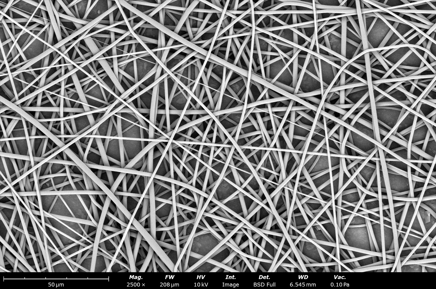
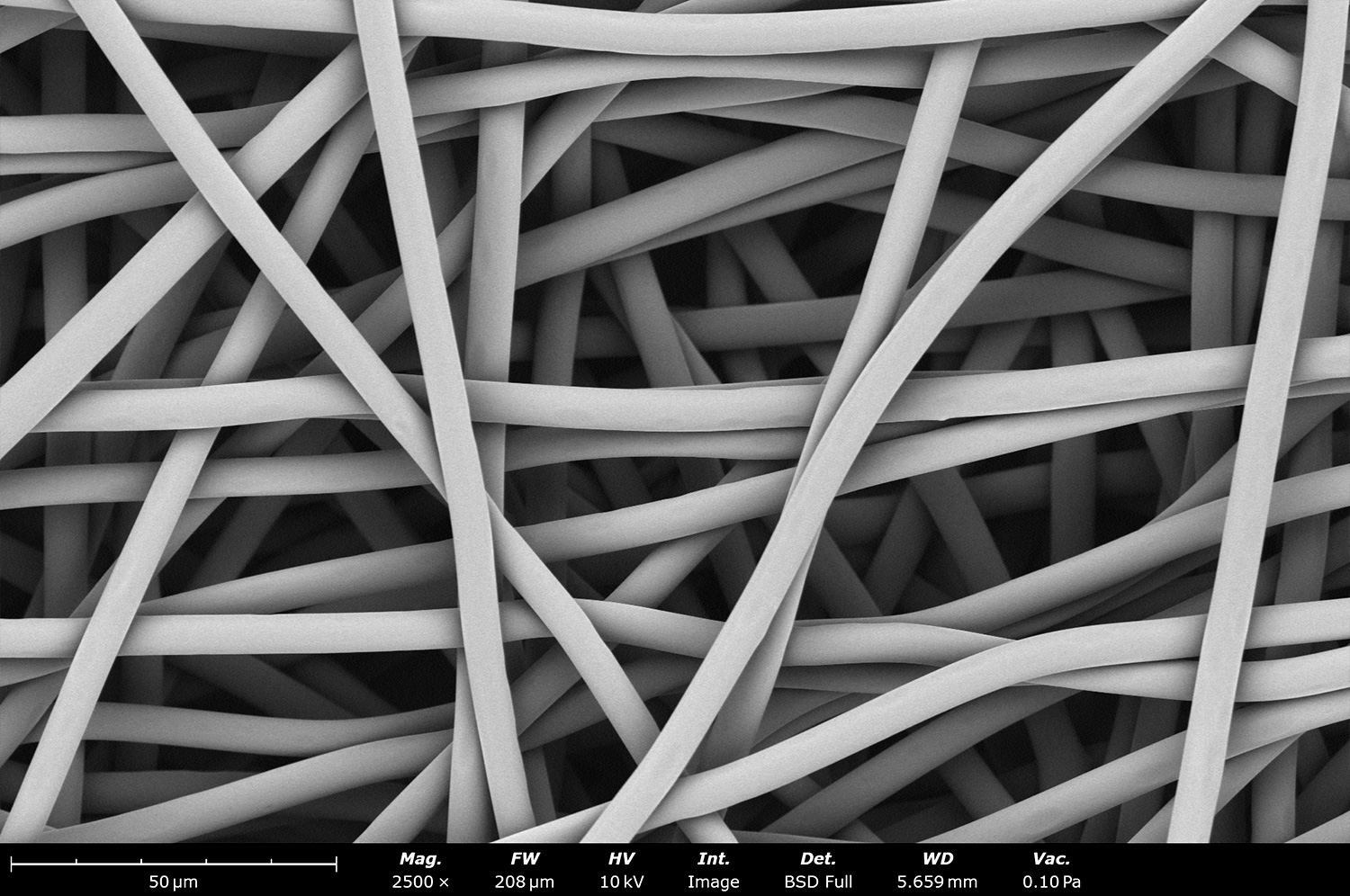
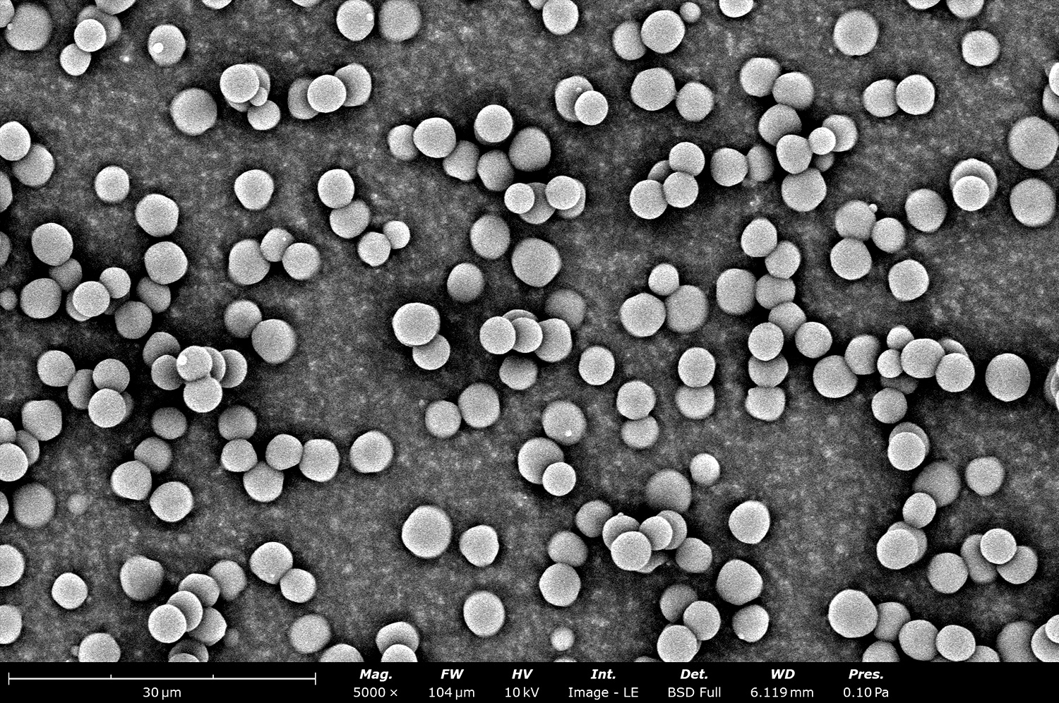
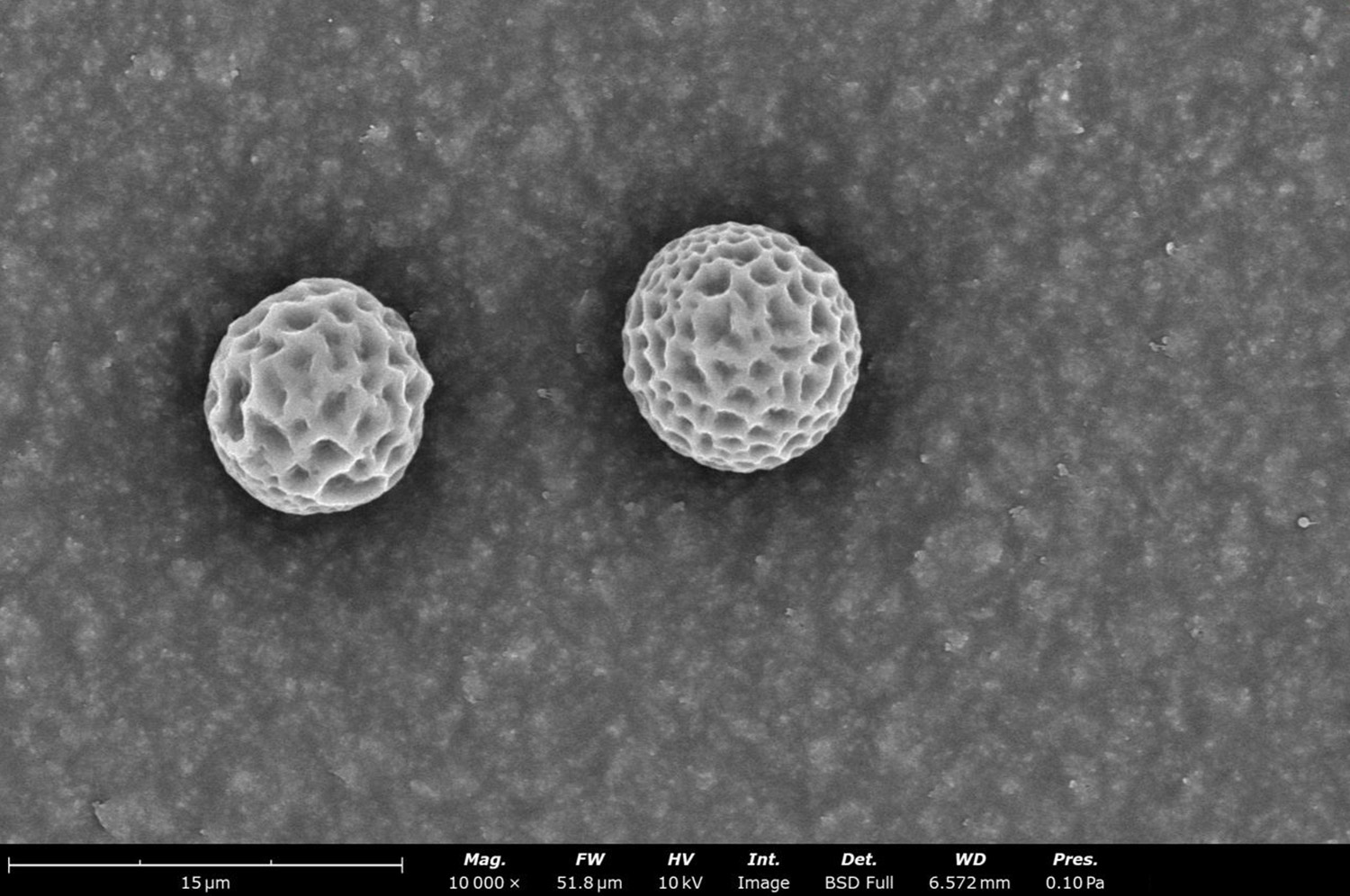
Figure 4. Effect on electrospun fibers and electrosprayed particles with different solvent systems. Electrospun fiber diameter for thermoplastic polyurethane (TPU) by changing the solvent system: a) HFIP only [FD = 1.52 ± 0.47 µm] and b) blended CHF:HFIP [FD = 6.54 ± 0.52 µm]. Effect on particle diameter for PCL (Mw ~ 50 kDa) with two solvent systems: c) acetic acid [PD = 3.72 ± 0.40 µm] and d) dichloromethane [PD = 9.04 ± 0.30 µm]. FD = fiber diameter and PD = particle diameter.

Viscosity and its Effects on Tubing Selection

Since the viscosity of non-Newtonian fluids changes based on the applied shear rate, the dimensions of the tubing and the pressure or linear force of the pump must be considered. Higher viscosity leads to increased friction and pressure drops within the tubing; to maintain desired flow rates, larger tubing or higher pump pressure may be required. In cases where smaller tubing is required to minimize dead volume when using expensive materials, the dispensing system will require higher linear forces. Knowing the linear force or pressure of the dispensing system along with the solution viscosity, users can choose a tubing diameter that prevents significant changes in fluid transportation. This decision becomes more impactful when scaling up the process and working with multiple linear injectors, since higher flow rates are required for consistent production.

Effect of temperature on viscosity

Temperature is another variable affecting solution viscosity, and ultimately, the samples generated with electrospinning and electrospraying processes. While it is well-known that elevated temperatures reduce solution viscosity, polymeric chain entanglement has been reported to be independent of solution temperature.⁹ While most solutions processed with these techniques are handled at room temperature, elevated temperatures can be useful when common organic solvents are not effective to make a homogeneous solution or when a decrease in viscosity improves polymer processability.

However, increasing temperature can modify key solution properties like viscosity, surface tension, and conductivity, which affect the tunability of fiber morphology. For example, the work done by Wang et.al. shows that increasing temperature from 32 to 89 °C for 6 wt% and 12 wt% polyacrylonitrile (PAN) in DMF effectively decreased viscosity and surface tension while increasing conductivity, resulting in a reduction of fiber diameter for both cases.⁹ It is important to note that this study utilized a solvent gas jacket of DMF to surround the needle. A similar study by Yang et.al. highlighted a similar trend for 15 w/v% PAN in N,N-Dimethylacetamide (DMAc) from 20 °C to 60 °C due to decrease in viscosity, but upon increasing temperature to 80°C, fiber diameter increased again. This increase can be attributed to not using solvent vapors around the needle, allowing the solvent to evaporate quicker at elevated temperatures. When using polyvinylpyrrolidone (PVP) in EtOH without a solvent gas jacket, a decrease in diameter is followed by an increase proportional to operating temperature.

The previous examples utilized polymers with high melting points. When using polymers with low melting points, such as PCL (T_m ~ 60 °C), fiber diameter trends are dependent on solvent selection. As shown by the work of Ramazani et.al., PCL solutions made with blended acetic acid and water (90:10 v/v%) resulted in a decrease in fiber diameter as temperature increased (25 to 45 °C). This is because the viscosity was reduced when the temperature increased.¹¹

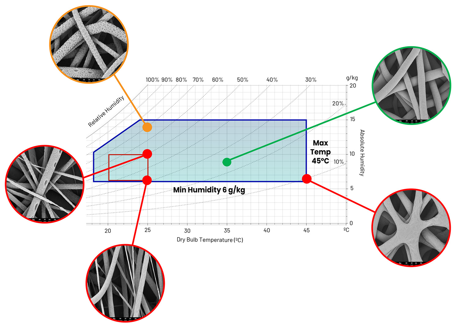
A study performed by Nanoscience Instruments explored the effects of PCL in solvents with high evaporation rates and low boiling points. For this, a 13.5 wt% PCL (M_n ~ 80 kDa) in CHF:MeOH (10:1) was produced under the tight temperature and relative humidity conditions achieved with the Fluidnatek LE-50 and its environmental control unit. Figure 5 shows a psychrometric chart used to properly correlate temperature, relative humidity and absolute humidity upon studying changes in environmental conditions for this PCL solution at sea level (atmospheric pressure = 101.325 kPa). When maintaining a constant temperature of 25 °C and increasing RH (30 to 70%), fiber diameter increases, and the surface becomes porous due to water droplets accumulating there during processing. Meanwhile, when temperature is increased from 25 °C to 35 °C, a uniform fiber morphology is obtained, and this is due to a rapid solvent evaporation when using a low RH of 25%. When further increasing the temperature to 45 °C (and 10% RH), fiber-fiber bonding defects can be seen due to a quicker evaporation rate of the solvent and the high temperature. A similar result can be seen even when using high boiler solvents like AA:W.¹³

The previous examples show how temperature increments have a direct effect in solution viscosity, electrospinnability, and eventually the resulting sample microstructure. Incrementing temperature can also influence mechanical properties, chain orientation, degree of crystallinity, crystal size and the final physical properties of the electrospun sample.¹³

Measuring viscosity

There are various ways to measure the viscosity of a solution, but in general, a viscometer or rheometer can be used. One of the most common methods to measure viscosity is using a rotational viscometer. It requires a sample volume as low as 2 mL, allowing the user to maximize sample volume for production or when expensive materials are used. A Peltier stage can maintain the solution temperature while a spindle rotates inside the solution to determine the torque; this is used to obtain the viscosity of the solution. Viscosity measurements are typically reported in units of centipoise (cP) along with the experiment’s temperature, shear rate, instrument, model, and processing parameters (spindle, cup, etc.).

Conductivity

Considering the physics that drive electrospinning and electrospraying, conductivity is a fundamental solution parameter. Conductivity must be optimized to properly generate fibers or particles; if it is too high or too low, effects such as arcing can disrupt the formation of fibers or particles. Also, conductivity relates to the charge density of the solution, which influences the elongation and stretching of the jet during electrospinning or electrospraying. Since solution conductivity also has effects on the ideal processing parameters and final sample properties, precisely quantifying it can help to optimize the process and ultimately improve batch-to-batch reproducibility.

Figure 6 is a general representation of how solution conductivity affects the electrospinning process and sample deposition area. Conductivity that is too low will cause the liquid to drip once the high voltage is applied, since there are not enough electrostatic forces to maintain a stable Taylor cone. Lower conductivity, but enough to start the process, results in less elongation and stretching of the polymer jet. These low conductivity solutions can lead to microstructures with beaded fibers and/or non-uniform fiber or particle diameter. Increasing solution conductivity with salt incorporation or using solvents with high dielectric constants will increase solution charge density, causing increased elongation and stretching during production. This results in a larger sample deposition area compared to solutions with lower conductivity.

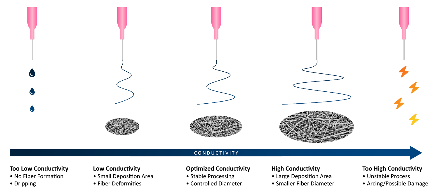
If the solution’s conductivity is further increased, the repulsive forces during sample production will also increase, which increases fiber stretching, decreases diameter, and increases sample deposition area. This is also true for electrospraying. If the conductivity is instead too high, the repulsive forces cause a variety of issues including unstable processing, arcing, lack of reproducibility, and possible damage to the instrument.

To evaluate the effects of an increment in solution conductivity, two samples were processed using the Fluidnatek LE-50. A 10 wt% PCL in HFIP solution acted as the control group, while 10 wt% PCL in HFIP with 10 wt% HEPES salt was used as the high conductivity solution. Figure 7 shows the effect on both solutions while controlling processing parameters. While the fiber diameter for the control group was uniform with a low standard variation (3.68 ± 0.16 µm), the solution with 10 wt% HEPES salt significantly decreased the fiber diameter (1.02 ± 0.50 µm). Sample deposition was also significantly affected during the electrospinning process. The control group had a small deposition width of 5.7 ± 0.1 cm across the substrate in the drum collector. Increasing solution conductivity with HEPES salt increased the deposition area to 17.9 ± 0.2 cm.

Figure 7. Microstructural changes and resulting sample macrostructure with different solution conductivities of 10 wt% PCL in HFIP. Microstructure of PCL: a) no salts (F_D = 3.68 ± 0.16 µm) and b) 10 wt% HEPES salt in solution relative to PCL content (F_D = 1.02 ± 0.50 µm); both at 10,00 X magnification. Final sample macrostructure: c) no salt (sample width = 5.7 ± 0.1 cm) and d) with 10 wt% HEPES salt (sample width = 17.9 ± 0.2 cm). Both samples developed under the same electrospinning conditions.

How to tune solution conductivity

Optimizing solution conductivity can improve process stability and give users greater control over parameters like fiber morphology and sample deposition area. This can be achieved with the use of additives like surfactants or salts, selecting different polymers or solvents, and altering the concentration of solution components.

Polymer Selection

The main polymer, a secondary polymer, or the use of co-polymers in solution will influence the solution’s conductive properties. The bonds of these polymers, which are alternating single-to-double and triple bonds, allow electrons to move through the backbone structure. Aromatic groups and atoms with free electrons in the structure can also help with solution conductivity. Examples of these types of polymers include polyaniline (PANI), polypyrrole (PPy), and poly(3,4-ethylenedioxythiophene) (PEDOT). Non-conductive polymer solutions like PCL can be doped with these polymers to improve solution conductivity and spinnability if the final application allows it.

Solvents

Solvent selection is another way to adjust solution conductivity. Typically, polar solvents are used to easily dissolve charged species and increase the solution’s ability to carry electrical current. Although it lacks a direct relationship with conductivity, solvents can be selected to have a high dielectric constant, which promotes ion dissociation and spinnability. This results in smaller fibers while maintaining a stable process. For example, Luo et.al. Showed that increasing the dielectric constant of a solution comprised of 10 wt% PCL (Mn ~ 80 kDa) in acetic acid, formic acid, or a mixture of the two results in a stable process and nanoscale fibers. The same study showed that using solvents that result in lower dielectric constants led to fiber diameters above thew nanoscale.¹⁴Solvent additives and quality can also affect the conductivity of the completed solution, which is why the same solvent grade should be maintained between batches. Deep eutectic solvents and ionic liquids can be added to adjust solution conductivity, improve spinnability, and achieve desired sample properties.

Additives

Additives, such as salts, ionic surfactants, or conductive nanoparticles, can be used to adjust solution conductivity. When selecting an additive, it is key to confirm that it can fully dissolve, mix fully, and stay homogeneous in solution without precipitating.

Disadvantages of increasing solution conductivity

Although increasing solution conductivity can improve sample morphology and spinnability, as shown in Figure 6, there are disadvantages to this that scientists will need to consider.

Post processing is required to leach out secondary polymers or additives such as salts. The main concern with leaching is that porosity can be introduced to an otherwise smooth sample. For applications that require a high surface area, this may be ideal, but otherwise, unintended porosity can cause mechanical property changes and other defects.
High conductivity tends to increase the sample deposition area. If the fibers or particles are not collected properly, which requires inducing a negative voltage on the collector, material will be deposited outside of the collector area and lost. When the solution contains expensive materials, this is especially important.
Increasing charge density can lead to an unstable electrospinning process. Depending on the solution’s conductivity, the process can also result in arcing as described in Figure 6, which can damage the equipment being used. Using professional electrospinning equipment such as Fluidnatek’s LE series will help prevent this, since they are equipped with arc detection and automatic shutoff.

How is solution conductivity measured?

Conductivity is measured with a combination of a conductivity meter and a probe. Standard probes can be used with green solvents, such as water, but when using acidic solvents or harsh additives, a specialized probe is required. It is also important to consider the probe’s range of conductivity and calibration procedures, especially with solution conductivities below 1 millisiemens per centimeter (mS/cm). Values are reported based on the selected ASTM standard reporting details, equipment details, and testing parameters such as analysis temperature.

Surface Tension

For the purposes of electrospinning and electrospraying, the surface tension of a polymer solution is what holds the solution at the needle tip. To generate fibers or particles, the surface tension must be overcome by applying high voltage, which can be seen in Figure 8a. The applied voltage must be high enough to deform the solution droplet into a conical Taylor cone, which enables fabrication of fibers or particles. This voltage is known as the critical voltage (V_c), which can be seen in Equation 1 and Figure 8b.¹⁵

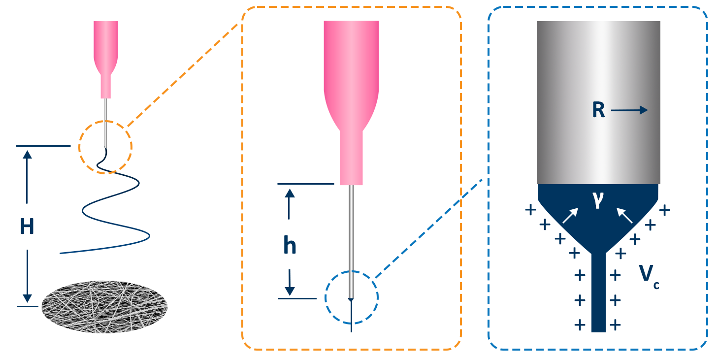
Figure 8. Visual representation of a) initiation of the electrospinning process when a voltage is applied at the needle, and b) diagram of all parameters involved to achieve a Taylor cone based on Equation 1.

V_c²

=

4H²

(

ln

2h

- 1.5

)

(0.117πγR)

h²

R

Equation 1
Where:
V_c is the critical voltage, kV
H is the distance between the needle and the collector, cm
h is the needle length, cm
R is the radius of the needle, cm, and
γ is the surface tension of the liquid, mN/m.

As shown in Equation 1, the surface tension of the solution and critical high voltage needed to initiate the electrospinning/electrospraying process are directly proportional. This means solutions with lower surface tension can be processed at lower voltages, which can be beneficial for both needle-based and needle-less electrospinning.

Effect of solution concentration and solvent selection on surface tension

One way to optimize surface tension of a solution is to adjust its concentration. This can result in an increase, decrease, or unchanged surface tension depending on the chemical interactions of the polymer and solvent. For example, the work done by Jarusuwannapoom et.al. shows that increasing the concentration of polystyrene from 10 to 30 w/v% in solvents like 1,2-dichloroethane, ethyl acetate and methylethylketone increased surface tension in solution. Meanwhile, when using solvents like dimethylformamide and tetrahydrofuran with the same polymer complex, the surface tension decreases with an increase in solution concentration.¹¹

If the molecular weight of the polymer is relatively short, surface tension will not be drastically changed. However, if the molecular weight is higher, more chain entaglements can occur, leading to a much larger effect on the solution’s surface tension. In the work done by Silva et.al., the effect of hydroxypropyl methylcellulose’s molecular weight on surface tension was studied. The researchers showed that using a low molecular weight maintained a surface tension between 25.0 to 25.3 mN/m, with concentrations varying from 1 to 6 w/v% using a solvent of ethanol:water (75:25). Meanwhile, when using the high molecular weight version, the surface tension increased from 24.9 to 26.1 mN/m from a concentration of 1 w/v% to only 2.5 w/v%.⁵

To see the effects of surface tension with a common biodegradable polymer used in tissue engineering and medical devices, Nanoscience Instruments performed a study of concentration changes using polycaprolactone (M_n ~ 80 kDa) in 1,1,1,3,3,3-hexafluoroisopropanol (HFIP). Figure 9a shows the surface tension changes of PCL in HFIP for concentrations ranging from 0 to 10 wt%. In this particular case, the surface tension tended to increase with an increase in concentration when compared to pure solvent. These results can also be used to indirectly evaluate solution stability over time in terms of viscosity changes. For this, a surface tension versus concentration calibration has to be performed, where significant changes between different concentrations are relevant. Electrospinning users without a viscometer can simply evaluate the surface tension of the solution over time to confirm it is stable, and that solvent evaporation has not occurred.

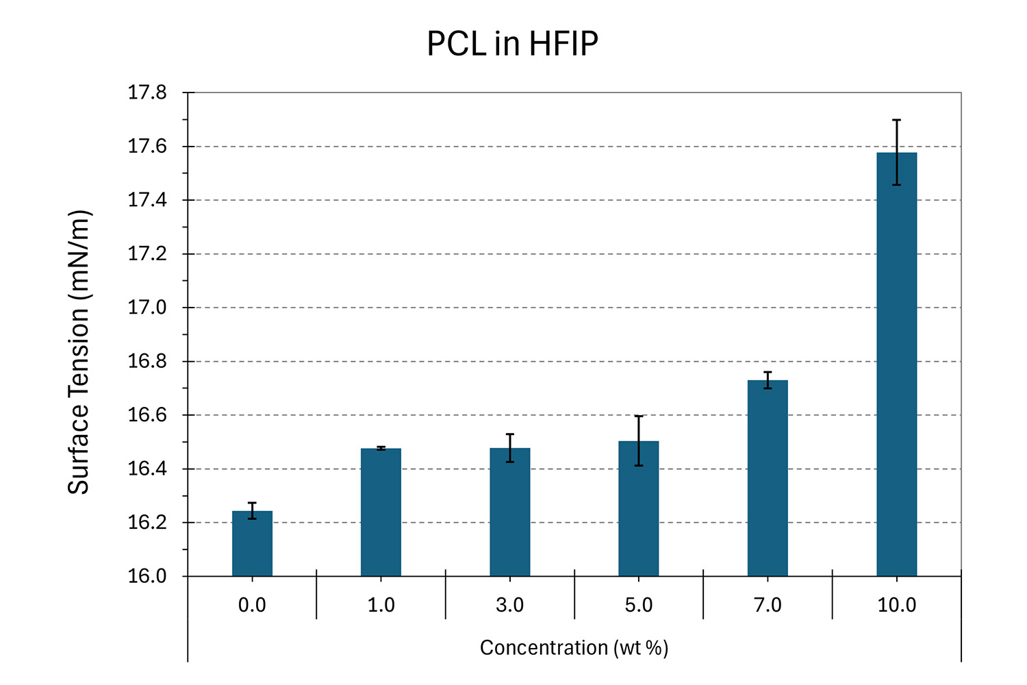
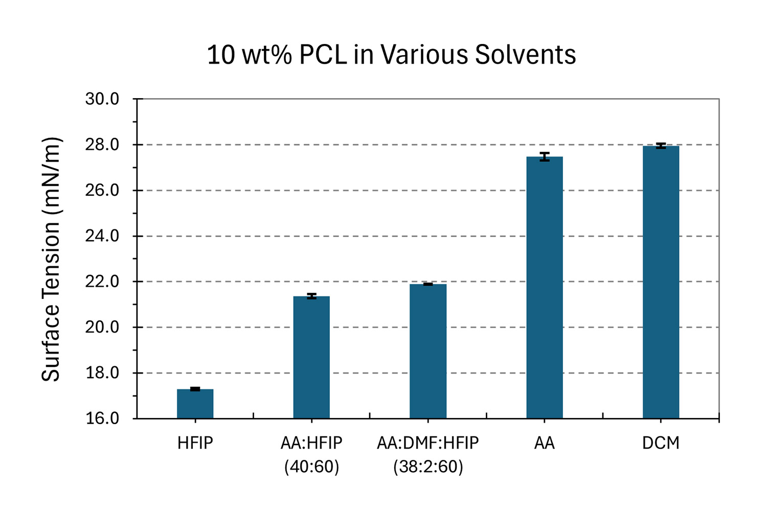
Figure 9. a) Effect of solution concentration on surface tension at different PCL in HFIP concentrations (analysis temperature of 22.3 ± 0.5°C), and b) surface tension changes based on solvent selection on 10 wt% PCL solutions (analysis temperature of 20.0 ± 0.2°C). Both results performed with an inverted pendant drop using a 22 Ga needle with the solution as the heavy phase and air as the light phase.

Depending on the polymer and additive(s) of interest in solution, co-solvents can be used to obtain a fully dissolved, homogeneous and well mixed solution. Co-solvent systems can also be advantageous for fine-tuning surface tension, resulting in a stable process during sample development. To showcase the effect of co-solvents, Nanoscience Instruments developed different solutions of 10 wt% PCL to see the effects on surface tension and microstructure. The surface tension results on these solutions are seen in Figure 9b. When using solvents with high surface tensions, like acetic acid (AA) and dichloromethane (DCM) (see Table 1), the surface tension of the 10 wt% PCL solution was 27.48 ± 0.17 and 27.95 ± 0.09 mN/m, respectively. Meanwhile, when combining AA and HFIP at a ratio of 40 to 60 by weight, the surface tension is reduced to 21.89 ± 0.02 mN/m. This last solution was spiked with dimethylformamide (DMF) to generate a solution with co-solvents of AA:DMF:HFIP at a ratio of 38:2:60 by weight, which slightly adjusted the surface tension to 21.89 ± 0.02 mN/m.

The effects of solvent selection on the microstructure for 10 wt% PCL are shown in Figure 10. All electrospinning parameters were kept constant except for voltage, as it was adjusted for each solution to maintain a stable Taylor cone during sample development. Microscale fibers were obtained when using HFIP (Figure 10a) as the surface tension was only 16.6 mN/m (Table 1), and beaded nanoscale fibers were obtained with AA (Figure 10d, surface tension of 27 mN/m). These beaded fibers are not ideal for most applications and can be easily removed by using a co-solvent system. Figure 10c shows a bead-free microstructure using AA:HFIP (40:60). This is attributed to improved solution processability during sample development due to a decrease in surface tension and boiling point, as well a slight increase in vapor pressure and dielectric constant. The fiber diameter can be further narrowed down with a slight addition of DMF, which increases the dielectric constant in solution (Figure 10d).

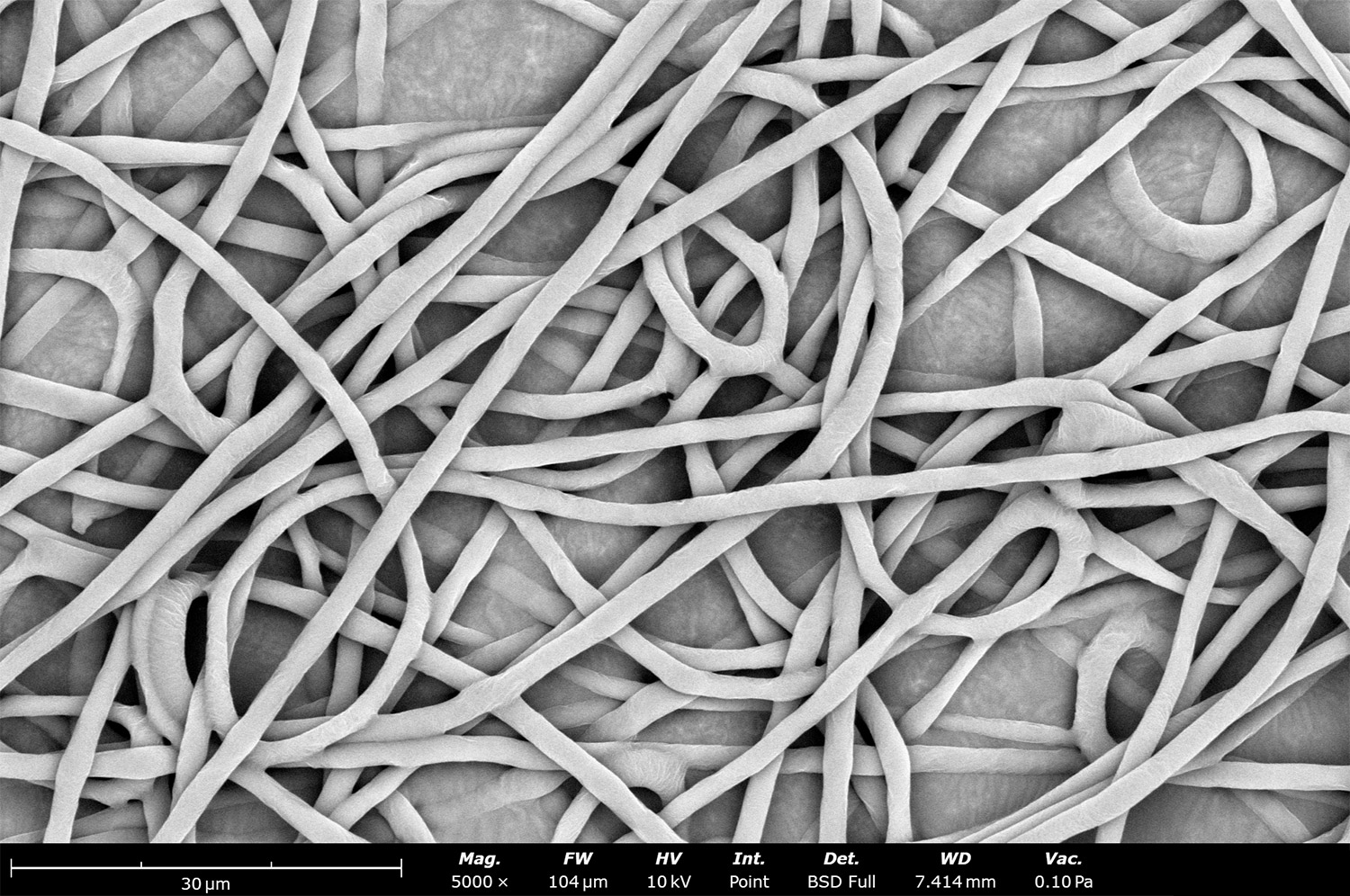
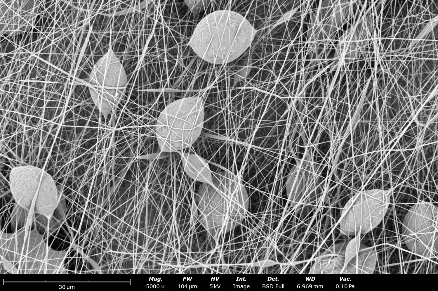
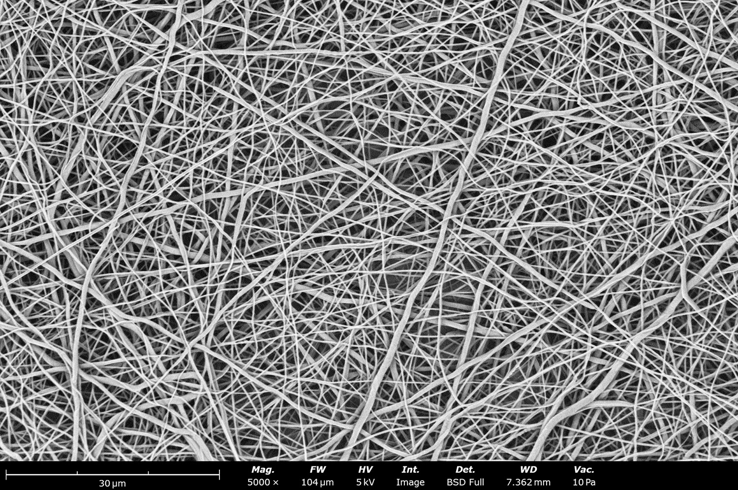
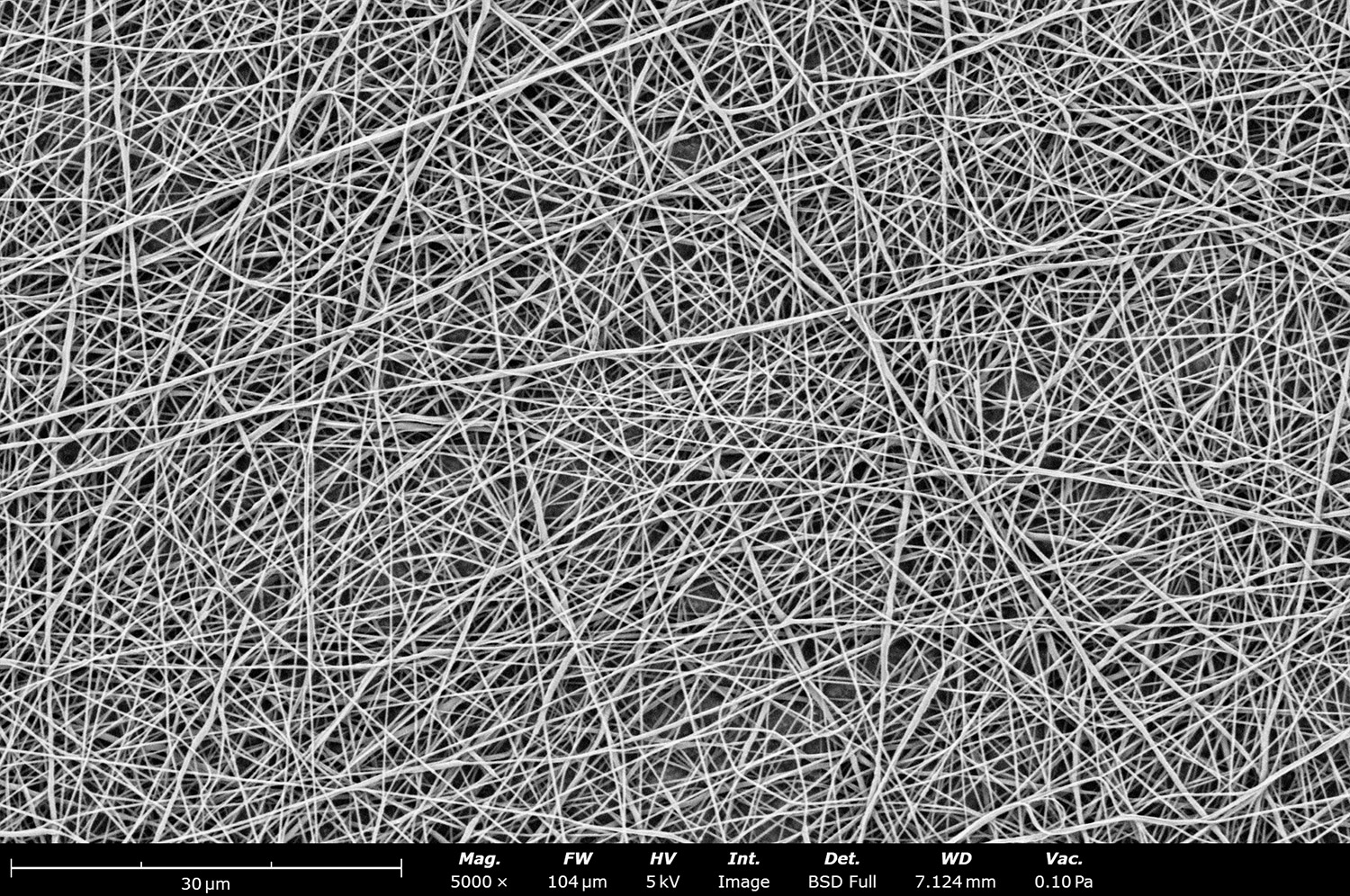
Figure 10. Effect of solvent selection on fiber diameter using PCL (M_n ~ 80 kDa) in various solvents: a) HFIP, b) AA, c) AA:HFIP (40:60), d) AA:DMF:HFIP (38:2:60), e) DCM, all at a magnification of 5,000 X, and f) average fiber diameter analysis. Note that electrospinning parameters were kept similar between each sample to easily compare effect on surface tension (flow rate of 2 mL/h, needle-to-collector distance of 13 cm, temperature of 25.0 ± 0.5°C and relative humidity of 40 ± 2%).

Lastly, a DCM-based solution was also processed to show how a solution with a high surface tension, and relatively similar to the AA version, can still achieve micro-scale fibers. This is mainly due to the solvent’s low boiling point and high vapor pressure (Figure 10e). It is important to note that all these microstructures were obtained with similar electrospinning parameters to better compare surface tension changes.

Effect of additives on surface tension

Using additives in solutions for electrospinning/electrospraying is common, since they can help solubilize other materials, stabilize vaccine formulations, incorporate antimicrobial properties, and even improve controlled release of drugs.¹⁶ Examples of additives include organic and inorganic salts, secondary polymers, nanoparticles, and surfactants. Work done by Wu et.al shows how using surfactants, specifically polysorbate 80, can be used to reduce surface tension, improve Taylor cone stability, and prevent macrostructural defects in poly(L-lactic-co-ε-caprolactone) (PLCL) scaffolds used as artificial blood vessels.¹⁷

Effect of temperature on surface tension

For electrospinning, there are two main temperatures to consider: the temperature of the chamber during the electrospinning process (see Figure 5), and the temperature of the solution itself. With the latter, increasing temperature results in a reduced surface tension and lower required operating voltage. This process is also known as hot-solution electrospinning, where temperatures typically range from 30 to 120 °C depending on the polymer, solvent, and additives used in the solution. Increasing the solution temperature can also allow the user to obtain smaller fiber/particle diameters and reduce the presence of beaded fibers.

One potential drawback of hot-solution electrospinning is that materials that are thermosensitive, like peptides and proteins, can denature and lose their functional properties. Hot-solution spinning can also increase the evaporation rate, which leads to larger fiber diameters and potential needle clogging. Heat can also lead to accidental co-polymer generation when two or more polymers are in solution.

Effect of scalability with solution surface tension

When a solution or product is ready to be scaled up to larger electrospinning/electrospraying systems, multi-needle configurations and increased flow rates are typically required. A common misconception is that if the process for a single needle is stable over time, it can be easily scaled up by increasing the needle count. However, there are more factors to consider. For example, if the process for one needle operates at a voltage of +25 kV, but the system’s power supply has a maximum of +30 kV, scaling up will be challenging, although not impossible. Solution surface tension is also key to consider; solutions with lower surface tensions can be processed at lower voltages, allowing users to increase the needle count and solution flow rate more easily.

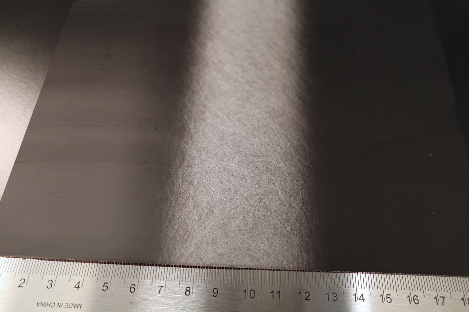
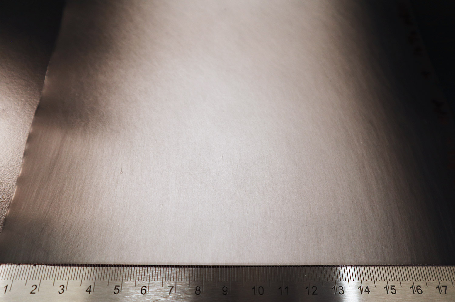
Since the surface tension of water tends to be higher, being around 72.8 mN/m at 20 °C, the voltage required to process water-based solutions will also be higher. Co-solvents are one option to decrease surface tension if the materials are compatible. For example, ethanol is a co-solvent of choice for most water-based solutions since its surface tension is only 22.1 mN/m at the same temperature. Another polar solvent choice for its surface tension is HFIP (16.6 mN/m at 20 °C). As seen in Figure 9a, the surface tension of PCL in HFIP at different concentrations is relatively low (<18 mN/m at ~22 °C) when compared to other solutions, making the scale up process easier and quicker. An example of this process is shown in Figure 11a with 60-needles and using the Fluidnatek LE-500 under tight environmental conditions and employing the roll-to-roll collector. An example of scaling a solvent with high surface tension is shown in Figure 11b, where a solution of 8 wt% polyacrylonitrile in dimethylformamide has been scaled up to 20 needles.

Figure 11. Scale up process of two different optimized solutions generated using the Fluidnatek LE-500 equipment under tight environmental conditions after solution optimization: a) polycaprolactone in hexafluoroisopropanol using 60-needles and processed for over two hours, and b) polyacrylonitrile in dimethylformamide using 20-needles.

How to measure surface tension in a polymeric solution

There are multiple ways to measure the surface tension of a polymeric solution, but generally, tensiometers are used. Force tensiometers measure the forces exerted on a specially-designed probe, while optical tensiometers analyze the shape of a droplet with a camera and analytical software. The latter process, also known as a contact angle measurement, can determine the hydrophobicity of the final sample.

There are multiple factors to consider when selecting a surface tension analysis method for polymeric solutions. Typical solutions used in electrospinning and electrospraying use solvents with low surface tensions (see Table 1), which includes values below 30 mN/m when using organic solvents. Although the exact value will depend on multiple factors like concentration of polymer, solvents, co-solvents, and additives, having an expected idea of the surface tension can give scientists an idea of which measurement methods might be best for their solution. Other factors that might affect this decision include available sample volume, solvent toxicity, and evaporation rate.

Surface Tension (Via Wilhelmy Plate)

A force tensiometer could be a good fit if enough solution is available, since measurements of this type require anywhere from several milliliters of solution up to 50 mL depending on the dimensions of the probe (Figure 12a and 12b). Also, if the measurement is performed with a Du Noüy Ring, the density of the solution must be known. For other probes, such as the Wilhelmy plate or a platinum rod, the solution density does not need to be known. To be a good candidate for force tensiometry, solutions should be stable and highly viscous.

This method should be performed inside of a fume hood, since the testing area of the force tensiometer is open to the lab environment. Surface tension measurements are typically reported with units of milli newton by meter (mN/m) along with the analysis temperature, probe type and dimensions, and model of instrument used.

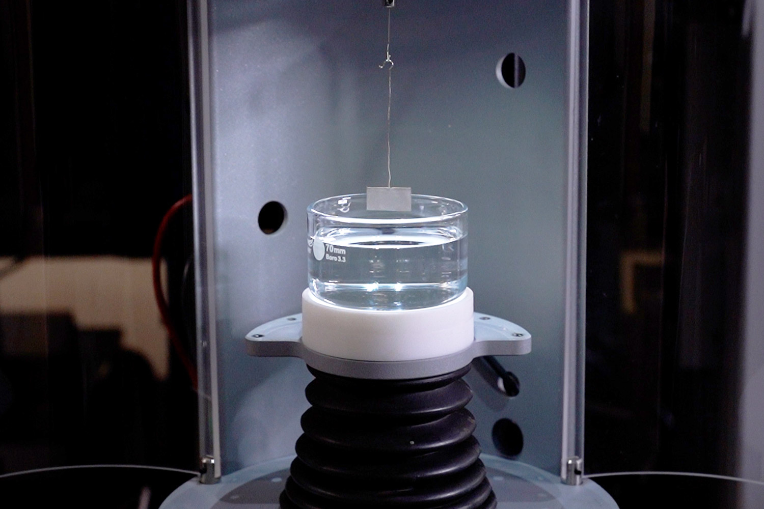
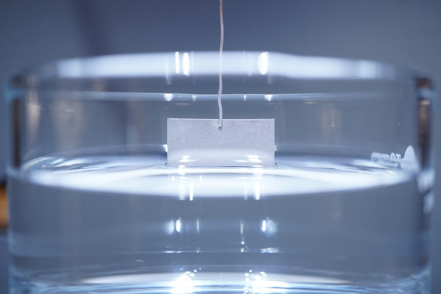
Figure 12. a) Experimental setup for a force tensiometer from Biolin using a Sigma 701 and a Wilhelmy plate, and b) close up image on the surface tension analysis for pure hexafluoroisopropanol.

Surface Tension (via Pendant Drop)

Pendant drop analysis, which can be performed with optical tensiometers, involves the use of a dispensing tip or needle to measure the surface tension of a droplet through image fitting software. A typical setup for this method is shown in Figure 13, along with its fitted analysis. Solutions with low surface tension (< 30 mN/m) can experience a low capillary rise with certain dispensing tips, wetting the side of the dispenser and affecting the measurement. Figure 14 demonstrates how pure HFIP (surface tension of 16.6 mN/m at 20°C) tends to wet the side of all dispensing tips and stainless-steel needles used. To combat this, fluorinated based tips such as perfluoroalkoxy alkanes (PFA) or polytetrafluoroethylene (PTFE)¹⁹ should be used.

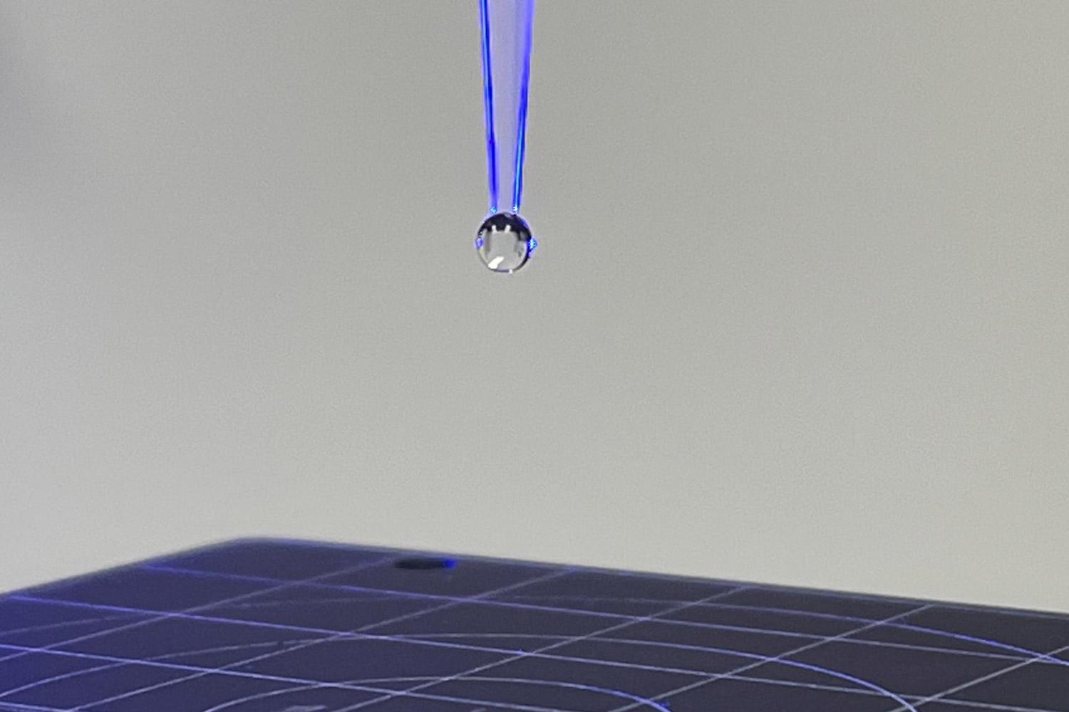
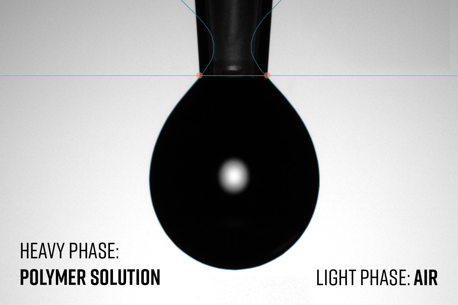
Figure 13. Surface tension measurement on a polymer solution using the Attension Theta Flow equipment using the for a pendant drop analysis (a) and its fitted analysis (b).

Figure 14. Polycaprolactone in hexafluoroisopropanol at different concentrations being dispensed through a wide orifice polypropylene tip through air displacement: a) 3.5 wt% and b) 10 wt%. Due to the low surface tension and high viscosities of the solutions the drop continues to flow and surface tension analysis was not possible with regular pendant drop analysis using air displacement.

Low surface tension, high viscosity, high density, and poor dispensing configuration can all cause defective drop formation. For example, Figure 15 shows pendant drop measurements using PCL in HFIP at two different concentrations (3.5 wt% and 10 wt%). In both instances, the solution was displaced using an air displacement system. Due to the low surface tension, high viscosity, and solution density above 1.5 g/mL, both solutions tended to drip, preventing accurate pendant drop measurements.

Figure 15. Polycaprolactone in hexafluoroisopropanol at different concentrations being dispensed through a wide orifice polypropylene tip through air displacement: a) 3.5 wt% and b) 10 wt%. Due to the low surface tension and high viscosities of the solutions, the drop continues to flow, and surface tension analysis was not possible with regular pendant drop analysis using air displacement.

If the solvent or solvent mixture in solution has a high surface tension, but shows low volatility properties (high boiling point and low vapor pressure), the pendant drop method can still be used. This is because solutions with highly volatile solvents will tend to evaporate too quickly, causing solidification of the solution drop and inconsistent surface tension readings. Figure 16 shows a 10 wt% polycaprolactone in dichloromethane during pendant drop analysis using a standard polypropylene tip. It is clear that the solvent has evaporated too quickly, and the solution has started to solidify.

For surface tension measurements with pendant drop, the density of the solution must be known. The volume needed to perform the measurements will depend on the size and quantity of droplets, but typically stays within 5 – 20 μL per sample.¹⁹ Surface tension measurements are typically reported with units of milli newton by meter (mN/m) along with the analysis temperature, probe type and dimensions, and model of instrument used.

Surface Tension ( via Inverted pendant drop)

An inverted pendant drop, as shown in Figure 17, involves dispensing and suspending an air bubble inside the solution of interest. Since greater viscous forces are exerted by the solution than by the atmosphere, it is crucial to let the air bubble stabilize before taking a measurement. Waiting more than 30 seconds before doing the analysis is typically recommended. To confirm stability, a live analysis can be performed to see if the volume and surface tension of the air bubble are changing over time. Inverted pendant drop analysis does not require a special chemistry of needle, but it needs to be hooked in shape, and the solution must be transparent.

The volume of solution required to perform this test depends on the dimensions of the cuvette used, which could be less than 2 mL. Covering the cuvette during analysis will minimize exposure to solvents. Bubbles around the analysis area should be avoided to prevent interference with the measurement. The density of the solution must be known to obtain surface tension through optical imaging.

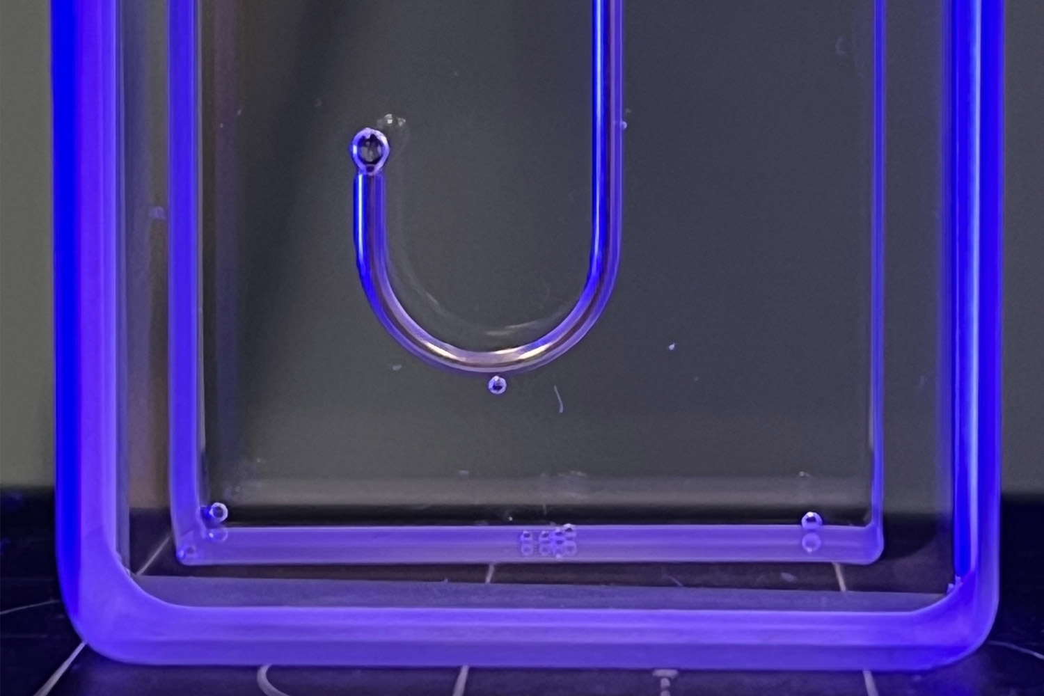
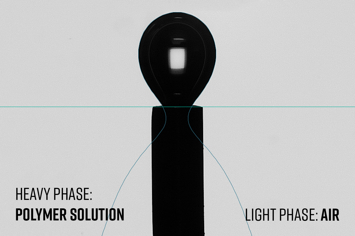
Figure 17. Inverted pendant drop analysis for 10 wt% polycaprolactone in hexafluoroisopropanol using a 22 Ga inverted needle (a) along its fitted analysis (b).

Inverted pendant drop is ideal for solutions with a low boiling point, high vapor pressure, or high viscosities. Since it is not as complicated or time consuming as the regular pendant drop, it is a popular option for testing challenging polymeric solutions. Surface tension measurements are typically reported with units of milli newton by meter (mN/m) along with the analysis temperature, probe type and dimensions, and model of instrument used.

Solution Age

Solution age is a significant factor in electrospinning and electrospraying processes since it affects both solution and processing parameters. Inconsistent solution age will lead to variability between batches and a lack of reproducibility. The key factors to consider when maintaining material stability over time are discussed below with regard to both the raw materials and the solution prepared with them.

Storage Vessel

If a storage container is not properly closed, solvents can evaporate over time and cause a change in polymer concentration. This then affects solution viscosity, conductivity, and surface tension (Figure 9a). Once these solution parameters change, the processing parameters must also be adjusted to obtain a stable Taylor cone.

Since solutions are often stored in the same syringe or vessel they were prepared in, which cannot be properly sealed, this is a common issue among electrospinning scientists. Depending on the solvent used, the rubber plunger of a syringe can swell over time, causing concentration changes. Sometimes parafilm is used to prevent evaporation, but this is not stable for long periods of time.

Ideally, a fresh solution should be prepared for each batch and used within 1-3 days, depending on the solvent. For solutions that need to be stored, it is important to confirm that the vessel is properly sealed and that no solvent can escape over time. This will extend the lifetime of the solution. It can also be beneficial to study how the solution’s properties generally change over time.

Color Changes

Color changes are a simple indicator of stability over time. Some materials can be light sensitive and break down over time, causing the solution color to change and indicating an unstable chemical structure. For these materials, amber glass containers are used and stored in the dark.

Another cause of color change is a reaction between the solvent and polymer in solution. A study done by Li et.al. showcased how thermoplastic polyurethane (TPU) at a concentration of 5 w/v% has a gradual color change from clear to orange-red, along with a flocculent precipitate, when using a DMF:THF (1:1) system. The researchers also showcased when selecting chloroform and 2,2,2-trifluoroethanol (1:1) the solution remains clear, suggesting this solvent system maintains a stable chemical structure for TPU for over 144 hours.¹²

Humidity

Hygroscopic materials like to attract and absorb moisture from their surroundings. Polymers, solvents, and even additives could all be classified as hygroscopic depending on their properties. Knowing if a chosen material is hygroscopic is important to prevent increased water content over time. This classification can be found on the safety data sheet of the raw material. Storing raw materials under an inert environment, or using a vessel with desiccant, is recommended for those types of materials.

Temperature

The temperature during solution preparation and storage, along with the time exposed to these temperatures, should be evaluated. Depending on the polymer, solvent, and additives in the solution, the raw materials could be reacting and changing properties over time.

For example, a study done by Ramazani et.al. explored the effect of temperature and exposure time on polycaprolactone (M_n ~ 80 kDa) dissolved in acetic acid. The research demonstrated how acetic acid can break down the polymer chain length onto smaller sections at various temperatures (25 to 55°C) and long exposure times(3 to 15 hours), decreasing its molecular weight to less than 10 kDa depending on the condition studied.¹³ This is valuable information; for polymers with lower molecular weights, the concentration will remain the same if the solution is stored properly, but the viscosity will be reduced over time, affecting the morphological and structural properties of the solution.

Controlling the temperature of the solution storage area will prevent drastic property changes. Using a fridge can be a good way to minimize evaporation, but it might not prevent it entirely, depending on the solvent volatility. For storing over long periods of time, the user should carefully study how temperature affects the solution being stored.

Use of Additives

Additives can potentially improve solution stability over time, but they might have effects on other properties. For example, organic salts can be used to improve stability, but conductivity will also be affected. This means that the use of additives in solution varies depending on application needs. Additives in solution can experience property changes as well, which affect the final solution.

Storage Time

When long-term storage is required, stability testing should be performed on the solution to characterize its concentration, viscosity, conductivity, and surface tension, among others. This is key to know if the solution changes over time. It is important to note that this differs from an accelerated study, where the sample is exposed to elevated temperatures to quickly degrade over time. Instead, the true storing conditions and how they impact the final processing parameters should be studied.

Generally, good practices include using a solution as fresh as possible when processing electrospun fibers or electrosprayed particles. With a known flow rate and processing time, you can calculate the volume of solution needed to prepare necessary quantities and prevent waste. This is especially important when using low boiling point solvents with high vapor pressures that can evaporate quickly over time. For solutions with high boiling points and low vapor pressures, using the solution within 3 days is recommended, but the solution still needs to be evaluated to confirm stability. Changes in concentration will affect solution properties and ultimately the microstructure of the sample. For improved reproducibility, a full solution characterization and future analysis on fresh batches is recommended to maximize productivity.

Conclusion

To achieve batch-to-batch consistency between samples developed through electrospinning and electrospraying, solutions must be fully dissolved, well mixed, and homogenous. Ideally, a full characterization of the sample, including solid content, viscosity, conductivity, and surface tension, should be performed. Solutions should be as fresh as possible to minimize variations between samples, but if needed, solutions can be stored over long periods of time, given that a long-term stability analysis confirms a lack of significant property changes. Once all these components are taken into consideration, and the process parameters have been optimized, electrospinning/electrospraying scientists will have a consistent product with minimal variability in microstructure, as shown in Figure 18.

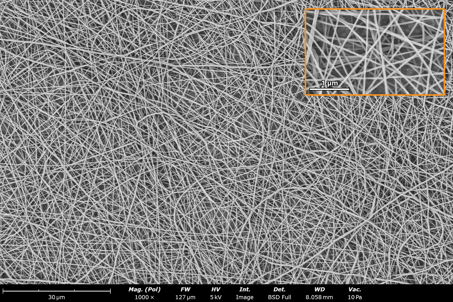
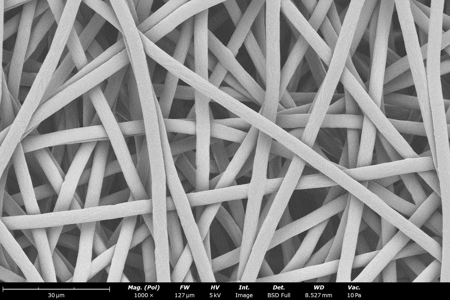
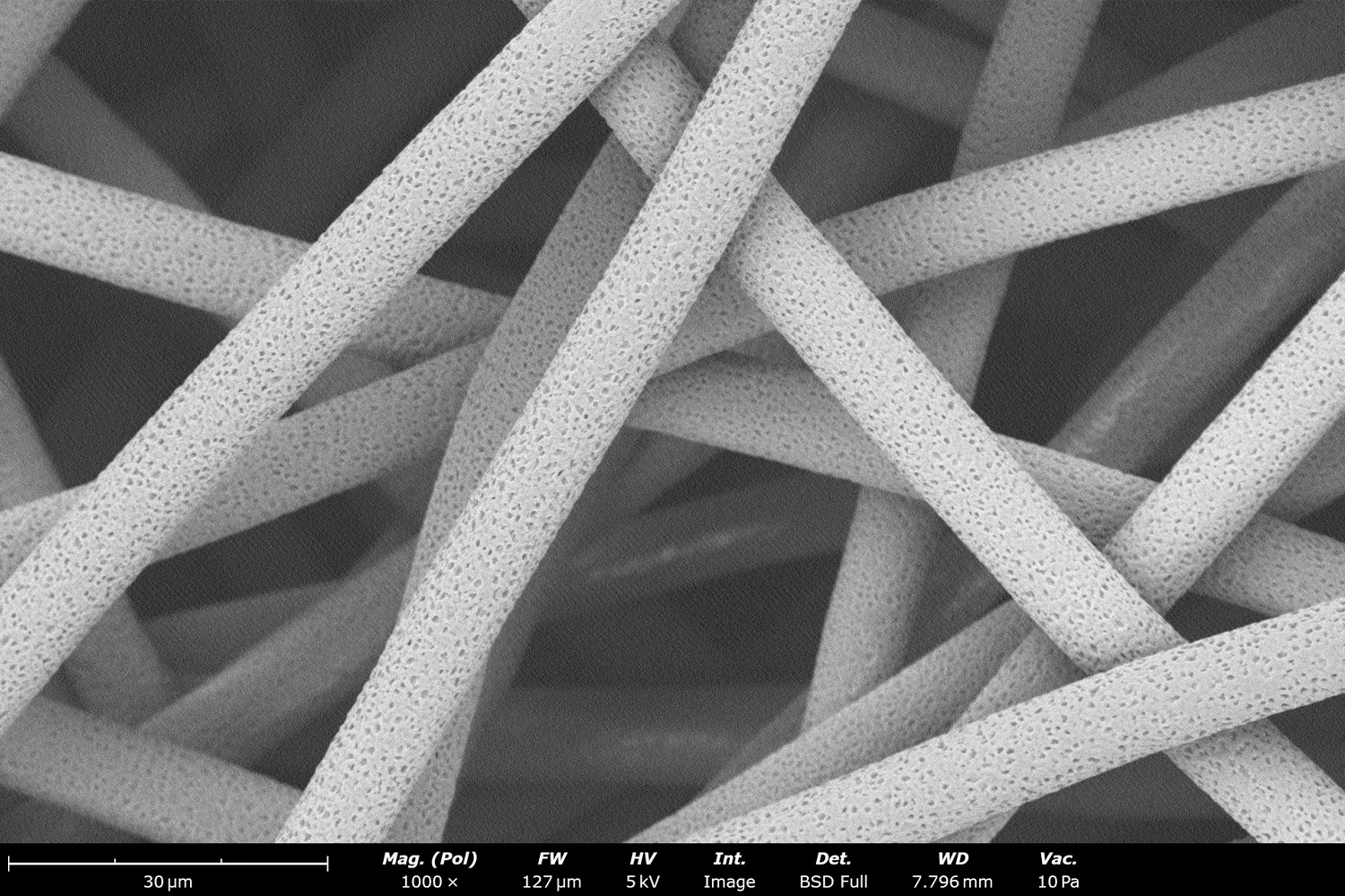
Figure 18. When considering all solution processing parameters mentioned throughout the document, along with tightly controlling all processing parameters with the Fluidnatek equipment, the microstructure of PCL can be optimized in various solvents to achieve fibers at different diameters: a) nano scale with AA:DMF:HFIP (38:2:60), b) micron with HFIP and c) micron scale with DCM. All images at a magnification of 1,000 X; scale bar of inset image is 1 µm.

References

ASTM Standard, D5226-21, “Standard Practice for Dissolving Polymer Materials”, ASTM International, West Conshohocken, PA, 2021, DOI: 10.1520/D5226-21, astm.org

Surface Tensions of Available Pure Substances. Accessed: January 30, 2025. https://materials.springer.com/interactive/overview?propertyId=PhysProp-8pugvrr1etqsf8rvbqr66e4l8e8cciga

Salimbeigi, G., Cahill, P.A. and McGuinness, G.B., Solvent system effects on the physical and mechanical properties of electrospun Poly(ε-caprolactone) scaffolds for in vitro lung models, Journal of the Mechanical Behavior of Biomedical Materials, Volume 136, 2022, https://doi.org/10.1016/j.jmbbm.2022.105493.

He, Z.; Rault, F., Vishwakarma, A., Mohsenzadeh, E. and Salaün, F., High-Aligned PVDF Nanofibers with a High Electroactive Phase Prepared by Systematically Optimizing the Solution Property and Process Parameters of Electrospinning. Coatings 2022, 12, 1310. https://doi.org/10.3390/coatings12091310

Silva, P.M., Prieto, C., Lagarón, J.M., Pastrana, L.M., Coimbra, M.A., Vicente, A.A. and Cerqueira, M.A., Food-grade hydroxypropyl methylcellulose-based formulations for electrohydrodynamic processing: Part I – Role of solution parameters on fibre and particle production, Food Hydrocolloids, Volume 118, 2021, https://doi.org/10.1016/j.foodhyd.2021.106761.

Zhang, W., Chen, J. and Zeng, H., Chapter 8 – Polymer processing and rheology, Polymer Science and Nanotechnology, Elsevier, 2020, Pages 149-178, ISBN 9780128168066, https://doi.org/10.1016/B978-0-12-816806-6.00008-X.

Kol, R., De Somer, T., D’hooge, D.R., Knappich, F., Ragaert, K., Achilias, D.S. and De Meester, S., State-Of-The-Art Quantification of Polymer Solution Viscosity for Plastic Waste Recycling, Chemical Upcycling of Waste Plastics, 2021, 14, 4071. https://doi.org/10.1002/cssc.202100876

Yang, G.Z., Li, H.P., Yang, J.H., Wan, J. and Yu, D.G. Influence of Working Temperature on The Formation of Electrospun Polymer Nanofibers. Nanoscale Research Letters. 2017; 12(1):55. https://doi.org/10.1186/s11671-016-1824-8.

Wang, C., Chien, H.S., Hsu, C.H., Wang, Y.C., Wang, C.T. and Lu, H.A. Electrospinning of Polyacrylonitrile Solutions at Elevated Temperatures. Macromolecules 2007 40 (22), 7973-7983. https://doi.org/10.1021/ma070508n

Unverzagt, L., Dolynchuk, O., Lettau, O. and Wischke, C. Characteristics and Challenges of Poly(ethylene-co-vinyl acetate) Solution Electrospinning. ACS Omega 2024 9 (16), 18624-18633. https://doi.org/10.1021/acsomega.4c01452

Jarusuwannapoom, T., Hongrojjanawiwat, W., Jitjaicham, S., Wannatong, L., Nithitanakul, M., Pattamaprom, C., Koombhongse, P., Rangkupan, R., and Supaphol, P. Effect of solvents on electro-spinnability of polystyrene solutions and morphological appearance of resulting electrospun polystyrene fibers. European Polymer Journal, 41 (3), 2005, 409-421. https://doi.org/10.1016/j.eurpolymj.2004.10.010.

Li, B., Liu, Y., Wei, S., Huang, Y., Yang, S., Xue, Y., Xuan, H., Yuan, H. A Solvent System Involved Fabricating Electrospun Polyurethane Nanofibers for Biomedical Applications. Polymer, 12 (12), 2020, 3038. https://doi.org/10.3390/polym12123038

Ramazani, S. and Karimi, M. Investigating the influence of temperature on electrospinning of polycaprolactone solutions. e-Polymers, 14 (5), 2014, 323-333. https://doi.org/10.1515/epoly-2014-0110

Luo, C.J., Stride, E. and Edirisinghe, M. Mapping the influence of solubility and dielectric constant on electrospinning polycaprolactone solutions. Macromolecules, 45 (11), 2012, 4669-4680. https://doi.org/10.1021/ma300656u

Wei, L., Chapter 1 – Electrospinning Theory, Wiley, 2024, Pages 1-13, ISBN 9783527841479, https://doi.org/10.1002/9783527841479.ch1

Nagaraj, K. and Kamalesu, S. State-of-the-art surfactants as biomedical game changers: unlocking their potential in drug delivery, diagnostics, and tissue engineering. International Journal of Pharmaceutics, 676, 2025. https://doi.org/10.1016/j.ijpharm.2025.125590

Wu, C., Wang. H., and Cao, J. Tween-80 improves single/coaxial electrospinning of three-layered bioartificial blood vessel. Journal of Materials Science: Materials in Medicine, 34 (6), 2023. https://doi.org/10.1007/s10856-022-06707-x

Biolin Scientific, Which tip or needle is most suitable for your liquid?. https://www.biolinscientific.com/blog/which-tip-or-needle-is-most-suitable-for-your-liquid

Biolin Scientific, Surface Tension Measurements. https://www.biolinscientific.com/measurements/surface-tension

Preparing & Characterizing Electrospinning Solutions

Table of Contents