Improved control and design of dental and orthopedic bone implants through simultaneous characterization of topography and contact angle
To ensure the safety and quality of medical implants, parameters such as the roughness, cleanliness, and wettability of the surface must be characterized. Because these properties are all coupled to some degree (for example, roughness may enhance the hydrophobic or hydrophilic effects of a surface), it may be insufficient to simply take a single value, such as the contact angle, to fully understand the state of the surface. By combining a topographical measurement with the contact angle, the corrected contact angle and surface energy can be obtained. These values can then be used to determine not only whether the roughness treatment has yielded the desired result, but also whether the surface is free of contaminants.
Why are topgraphy and contact angle measurements important to implant design?
The dental and orthopedic implant markets are multi-billion markets and continue to grow as modern medicine improves and people live longer. Common locations for these implants include hips, knees, spines, and jaws. Due to the load-bearing nature of these applications, many of the materials used in these applications are metals such as stainless steel, titanium, or titanium alloys. The wettability and roughness of the surface plays a large part in whether proteins and cells can attach to the surface and anchor the implant to the bone. Materials that exhibit moderately hydrophilic properties tend to also be conducive towards protein adsorption and subsequent cell attachment. However, overly hydrophilic materials show decreased cell attachment, suggesting that this parameter should be kept at an optimal level. [1]
Prior to implantation, it is common to roughen the implant at specific bone-contacting locations to ensure that osteocytes are better able to infiltrate pores and attach to surface features. The process where these osteocytes intermingle with the foreign material and help anchor it to the body is known as osseointegration and is known to improve the stability and overall success of the implant. [2, 3] Because implants are used inside the human body, their fabrication and processing steps are critically important to control and monitor. Surface treatments to increase wettability and roughness should be closely characterized throughout the manufacturing process to ensure that values are kept at prescribed levels and that no byproducts or contamination is present.
Optical tensiometry is a technique that measures the contact angle of a surface using a probe liquid. The contact angle provides information about the wettability, surface energy, and cleanliness of a surface. When combined with a topographical measurement, the contact angle of a perfectly flat surface can be determined. This unique feature offered by the Theta Flex system provides key insight and control in both research and production situations.
How is Attension Theta Flex with Topography Module use for Measuring Surface Free Energy and Roughness
Method and Results
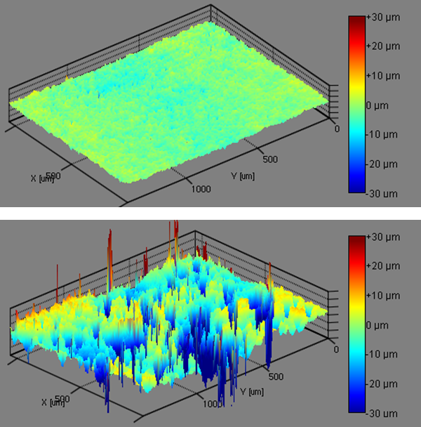
A Theta instrument equipped with the Topography Module was used to measure the surface free energy and roughness of titanium samples created by electrophoretic deposition (EPD). Different processing methods, designated Ti 1 and Ti 2, were used to achieve varying levels of surface roughness. Samples were first measured using the Topography Module, which utilizes a Fringe Projection Phase Shifting principle to measure the movement of fringes across a surface to determine the height of features on a surface.
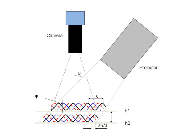
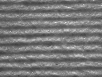
Figure 1 – Schematic of a fringe-projection phase shifting measurement and its corresponding optical surface
The technique utilizes an LED light and a slide with sinusoidal fringe patterns in line with a camera [4]. As the camera captures the movement of the fringes illuminated on the sample surface, each pixel is correlated with a specific phase shift and translated to a height through the OneAttension software.
Corrected contact angle was calculated using the following equations:


θm = the measured contact angle
θY = the Young’s contact angle, also known as the “corrected contact angle”
r = the roughness factor, defined as r=1 for a perfectly smooth surface, and r > 1 for a rough surface
Sdr = the area factor measured by the Topography Module, roughly defined as:

After the sample topography was measured, contact angle was measured using water and di-iodomethane. An automated XYZ stage was used to ensure that contact angle and surface roughness measurements were made on the exact same spot. Drops were applied by using an automated dispenser and disposable pipet tips. The measured and corrected contact angles were used to calculate the surface free energy (SFE) using the Owens, Wendt, Rable and Kaelble (OWRK) [7] and Acid-Base [8] methods. For more information about the different surface free energy theories and equations, please visit our technique pages on surface free energy.
Contact Angle Measurements with Water
| Sample | CA (STD) | CAc (STD) | Sdr (STD) |
|---|---|---|---|
| Ti 1 | 104.7 (6.9) | 101.4 (5.2) | 27.6 (4.8) |
| Ti 2 | 107.9 (2.3) | 102.6 (1.9) | 41.6 (8.2) |
| Ti 3 | 96.3 (2.3) | 93.5 (1.2) | 80.4 (6.4) |
| Ti 4 | 112.2 (1.8) | 101.9 (1.1) | 83.0 (6.3) |
Contact Angle Measurements Di-iodomethane
| Sample | CA (STD) | CAc (STD) | Sdr (STD) |
|---|---|---|---|
| Ti 1 | 56.7 (1.6) | 64.1 (2.4) | 26.3 (6.3) |
| Ti 2 | 49.8 (3.7) | 64.4 (3.4) | 51.1 (7.5) |
| Ti 3 | 56.9 (0.4) | 70.8 (0.9) | 66.0 (6.3) |
| Ti 4 | 46.7 (5.4) | 69.9 (1.9) | 95.6 (8.9) |
Surface Free Energy: OWRK
| Sample |
Surface Free Energy |
Corrected Surface Free Energy |
|---|---|---|
| Ti 1 | 30.5 | 26.8 |
| Ti 2 | 34.5 | 26.5 |
| Ti 3 | 31.2 | 25.3 |
| Ti 4 | 36.5 | 23.9 |
Surface Free Energy: Acid-Base
| Uncorrected Surface Free Energy (mN/m) | Corrected Surface Free Energy (mN/m) | |||||||
|---|---|---|---|---|---|---|---|---|
| Sample | Total | Dispersive | Acid | Base | Total | Dispersive | Acid | Base |
| Ti 1 | 35.4 | 41.8 | 1.0 | -3.3 | 32.3 | 36.0 | 0.8 | -2.2 |
| Ti 2 | 44.1 | 42.5 | 0.4 | 1.9 | 33.2 | 31.4 | 0.4 | 2.4 |
| Ti 3 | 33.9 | 34.8 | 0.6 | -0.8 | 26.0 | 25.1 | 0.7 | 0.6 |
| Ti 4 | 32.2 | 35.9 | 1.2 | -1.5 | 26.2 | 25.1 | 0.7 | 0.6 |
Discussion of Simultaneous Characterization of Topography and Contact Angle
Tables 1 and 2 show that the samples showed an increasing amount of roughness in the following order: Ti 1 < Ti 2 < Ti 3 < Ti 4. Table 3 effectively shows the important effect that roughness has on the material properties. The SFE measured using the OWRK method from the native samples shows a trend that almost correlates with the roughness of the samples, with the Ti 1 sample showing the lowest SFE and the Ti 4 sample showing the highest SFE. However, when the surface roughness is taken into account, the SFE trend is completely reversed. Ti 1 instead has the highest SFE and the EPD Ti 4 has the lowest SFE.
Drastic changes are also seen when measuring the titanium surfaces through the Acid-Base SFE method (Table 4). In this method, acidic, basic, and dispersive components are calculated for the material surface. Larger values in the acidic component suggest stronger interactions (i.e. better wetting) with basic liquids, and vice versa. For the uncorrected contact angle values, several samples had negative base values. However, when calculating the SFE using the corrected values, the basic values increased to the point where they were positive. These results show that surface roughness plays an important role in the surface properties of a material.
The ability to perform contact angle and surface roughness measurement on the exact same spot is currently offered only by the Theta Flex with Topography. The power of this combination of measurements is clearly shown in not just the contact angle correction data, but also the different conclusions drawn between the measured SFE and the corrected SFE. These fast, automated measurements should also in principle provide information about contaminants and other imperfections that may otherwise be undetected by a standard contact angle measurement. This is important not just in the development of current implant materials, but also in the development of next-generation products.
References
[1] R. E. Baier, “Surface behaviour of biomaterials: the theta surface for biocompatibility,” Journal of Materials Science: Materials in Medicine, vol. 17, no. 11, p. 1057, 2006.
[2] D. Buser, R. K. Schenk, S. Steinemann, J. P. Fiorellini, C. H. Fox and H. Stich, “Influence of surface characteristics on bone integration of titanium implants. A histomorphometric study in miniature pigs.,” Journal of biomedical materials research, vol. 25, no. 7, pp. 889-902, 1991.
[3] N. Meredith, “Assessment of implant stability as a prognostic determinant.,” International Journal of Prosthodontics, vol. 11, no. 5, 1998.
[4] S. Zhang and P. Huang, “High-resolution, real-time 3D shape acquisition.,” 2004 Conference on Computer Vision and Pattern Recognition Workshop. IEEE, p. 28, 2004.
[5] R. N. Wenzel, “Resistance of solid surfaces to wetting by water,” Industrial & Engineering Chemistry, vol. 28, no. 8, pp. 988-994, 1936.
[6] J. Peltonen, M. J. Järn, S. Areva and M. Lin, “Topographical parameters for specifying a three-dimensional surface,” Langmuir, vol. 20, no. 22, pp. 9428-9431, 2004.
[7] D. K. Owens and R. C. Wendt, “Estimation of the surface free energy of polymers,” Journal of Applied Polymer Science, vol. 13, no. 8, pp. 1741-1747, 1969.
[8] C. J. Van Oss, R. J. Good and M. K. Chaudhury, “The role of van der Waals forces and hydrogen bonds in “hydrophobic interactions” between biopolymers and low energy surfaces,” Journal of colloid and Interface Science, vol. 111, no. 2, pp. 378-390, 1986.